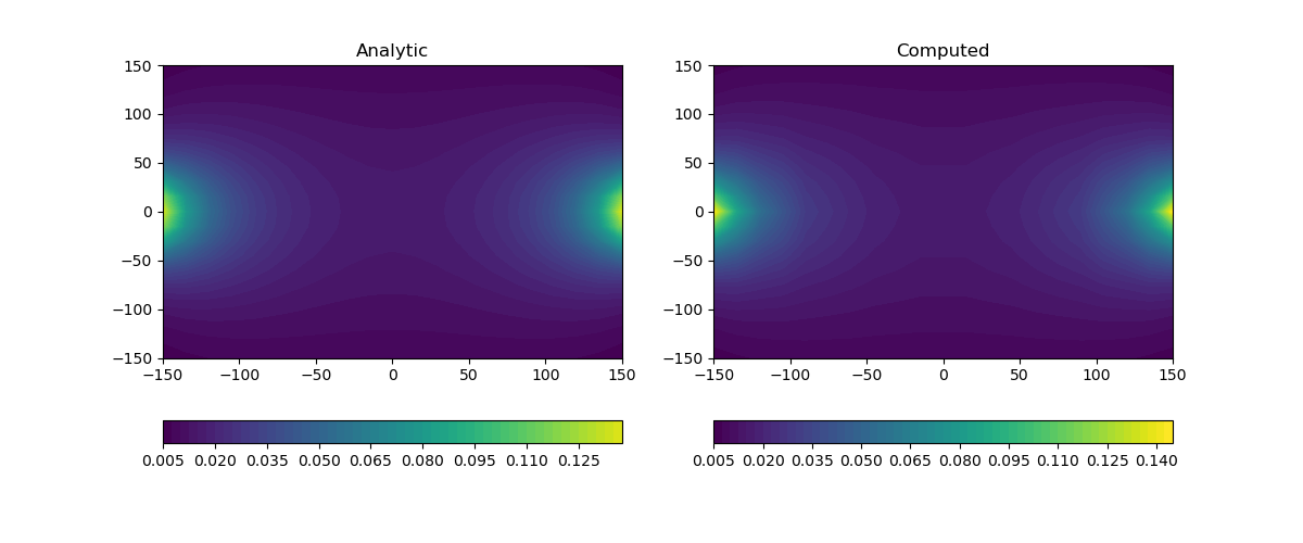
DC Analytic Dipole

Comparison of the analytic and numerical solution for a direct current resistivity dipole in 3D.

0.0646433348467705

import discretize
from SimPEG import utils
import numpy as np
import matplotlib.pyplot as plt
from SimPEG.electromagnetics.static import resistivity as DC

try:
    from pymatsolver import Pardiso as Solver
except ImportError:
    from SimPEG import SolverLU as Solver


cs = 25.0
hx = [(cs, 7, -1.3), (cs, 21), (cs, 7, 1.3)]
hy = [(cs, 7, -1.3), (cs, 21), (cs, 7, 1.3)]
hz = [(cs, 7, -1.3), (cs, 20)]
mesh = discretize.TensorMesh([hx, hy, hz], "CCN")
sighalf = 1e-2
sigma = np.ones(mesh.nC) * sighalf
xtemp = np.linspace(-150, 150, 21)
ytemp = np.linspace(-150, 150, 21)
xyz_rxP = utils.ndgrid(xtemp - 10.0, ytemp, np.r_[0.0])
xyz_rxN = utils.ndgrid(xtemp + 10.0, ytemp, np.r_[0.0])
xyz_rxM = utils.ndgrid(xtemp, ytemp, np.r_[0.0])


rx = DC.Rx.Dipole(xyz_rxP, xyz_rxN)
src = DC.Src.Dipole([rx], np.r_[-200, 0, -12.5], np.r_[+200, 0, -12.5])
survey = DC.Survey([src])
sim = DC.Simulation3DCellCentered(
    mesh, survey=survey, solver=Solver, sigma=sigma, bc_type="Neumann"
)

data = sim.dpred()


def DChalf(srclocP, srclocN, rxloc, sigma, I=1.0):
    rp = (srclocP.reshape([1, -1])).repeat(rxloc.shape[0], axis=0)
    rn = (srclocN.reshape([1, -1])).repeat(rxloc.shape[0], axis=0)
    rP = np.sqrt(((rxloc - rp) ** 2).sum(axis=1))
    rN = np.sqrt(((rxloc - rn) ** 2).sum(axis=1))
    return I / (sigma * 2.0 * np.pi) * (1 / rP - 1 / rN)


data_anaP = DChalf(np.r_[-200, 0, 0.0], np.r_[+200, 0, 0.0], xyz_rxP, sighalf)
data_anaN = DChalf(np.r_[-200, 0, 0.0], np.r_[+200, 0, 0.0], xyz_rxN, sighalf)
data_ana = data_anaP - data_anaN
Data_ana = data_ana.reshape((21, 21), order="F")
Data = data.reshape((21, 21), order="F")
X = xyz_rxM[:, 0].reshape((21, 21), order="F")
Y = xyz_rxM[:, 1].reshape((21, 21), order="F")


fig, ax = plt.subplots(1, 2, figsize=(12, 5))
vmin = np.r_[data, data_ana].min()
vmax = np.r_[data, data_ana].max()
dat0 = ax[0].contourf(X, Y, Data_ana, 60, vmin=vmin, vmax=vmax)
dat1 = ax[1].contourf(X, Y, Data, 60, vmin=vmin, vmax=vmax)
plt.colorbar(dat0, orientation="horizontal", ax=ax[0])
plt.colorbar(dat1, orientation="horizontal", ax=ax[1])
ax[0].set_title("Analytic")
ax[1].set_title("Computed")

print(np.linalg.norm(data - data_ana) / np.linalg.norm(data_ana))
plt.show()

Estimated memory usage: 18 MB