Note
Go to the end to download the full example code
Simulation with Analytic FDEM Solutions#
Here, the module SimPEG.electromagnetics.analytics.FDEM is used to simulate harmonic electric and magnetic field for both electric and magnetic dipole sources in a wholespace.
Import modules#
import numpy as np
from SimPEG import utils
from SimPEG.electromagnetics.analytics.FDEM import (
    ElectricDipoleWholeSpace,
    MagneticDipoleWholeSpace,
)

import matplotlib.pyplot as plt
from matplotlib.colors import LogNorm
Magnetic Fields for a Magnetic Dipole Source#
Here, we compute the magnetic fields for a harmonic magnetic dipole source in the z direction. Based on the geometry of the problem, we expect magnetic fields in the x and z directions, but none in the y direction.
# Defining electric dipole location and frequency
source_location = np.r_[0, 0, 0]
frequency = 1e3

# Defining observation locations (avoid placing observation at source)
x = np.arange(-100.5, 100.5, step=1.0)
y = np.r_[0]
z = x
observation_locations = utils.ndgrid(x, y, z)

# Define wholespace conductivity
sig = 1e-2

# Compute the fields
Hx, Hy, Hz = MagneticDipoleWholeSpace(
    observation_locations,
    source_location,
    sig,
    frequency,
    moment="Z",
    fieldType="h",
    mu_r=1,
    eps_r=1,
)

# Plot
fig = plt.figure(figsize=(14, 5))

hxplt = Hx.reshape(x.size, z.size)
hzplt = Hz.reshape(x.size, z.size)

ax1 = fig.add_subplot(121)
absH = np.sqrt(Hx.real**2 + Hy.real**2 + Hz.real**2)
pc1 = ax1.pcolor(x, z, absH.reshape(x.size, z.size), norm=LogNorm())
ax1.streamplot(x, z, hxplt.real, hzplt.real, color="k", density=1)
ax1.set_xlim([x.min(), x.max()])
ax1.set_ylim([z.min(), z.max()])
ax1.set_title("Real Component")
ax1.set_xlabel("x")
ax1.set_ylabel("z")
cb1 = plt.colorbar(pc1, ax=ax1)
cb1.set_label("Re[H] (A/m)")

ax2 = fig.add_subplot(122)
absH = np.sqrt(Hx.imag**2 + Hy.imag**2 + Hz.imag**2)
pc2 = ax2.pcolor(x, z, absH.reshape(x.size, z.size), norm=LogNorm())
ax2.streamplot(x, z, hxplt.imag, hzplt.imag, color="k", density=1)
ax2.set_xlim([x.min(), x.max()])
ax2.set_ylim([z.min(), z.max()])
ax2.set_title("Imaginary Component")
ax2.set_xlabel("x")
ax2.set_ylabel("z")
cb2 = plt.colorbar(pc2, ax=ax2)
cb2.set_label("Im[H] (A/m)")

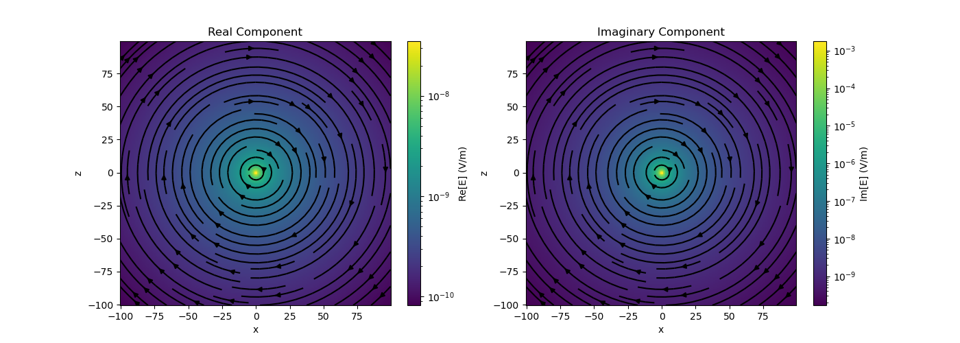
Electric Fields for a Magnetic Dipole Source#
Here, we compute the electric fields for a harmonic magnetic dipole source in the y direction. Based on the geometry of the problem, we expect rotational electric fields in the x and z directions, but none in the y direction.
# Defining electric dipole location and frequency
source_location = np.r_[0, 0, 0]
frequency = 1e3

# Defining observation locations (avoid placing observation at source)
x = np.arange(-100.5, 100.5, step=1.0)
y = np.r_[0]
z = x
observation_locations = utils.ndgrid(x, y, z)

# Define wholespace conductivity
sig = 1e-2

# Predict the fields
Ex, Ey, Ez = MagneticDipoleWholeSpace(
    observation_locations,
    source_location,
    sig,
    frequency,
    moment="Y",
    fieldType="e",
    mu_r=1,
    eps_r=1,
)

# Plot
fig = plt.figure(figsize=(14, 5))

explt = Ex.reshape(x.size, z.size)
ezplt = Ez.reshape(x.size, z.size)

ax1 = fig.add_subplot(121)
absE = np.sqrt(Ex.real**2 + Ey.real**2 + Ez.real**2)
pc1 = ax1.pcolor(x, z, absE.reshape(x.size, z.size), norm=LogNorm())
ax1.streamplot(x, z, explt.real, ezplt.real, color="k", density=1)
ax1.set_xlim([x.min(), x.max()])
ax1.set_ylim([z.min(), z.max()])
ax1.set_title("Real Component")
ax1.set_xlabel("x")
ax1.set_ylabel("z")
cb1 = plt.colorbar(pc1, ax=ax1)
cb1.set_label("Re[E] (V/m)")

ax2 = fig.add_subplot(122)
absE = np.sqrt(Ex.imag**2 + Ey.imag**2 + Ez.imag**2)
pc2 = ax2.pcolor(x, z, absE.reshape(x.size, z.size), norm=LogNorm())
ax2.streamplot(x, z, explt.imag, ezplt.imag, color="k", density=1)
ax2.set_xlim([x.min(), x.max()])
ax2.set_ylim([z.min(), z.max()])
ax2.set_title("Imaginary Component")
ax2.set_xlabel("x")
ax2.set_ylabel("z")
cb2 = plt.colorbar(pc2, ax=ax2)
cb2.set_label("Im[E] (V/m)")
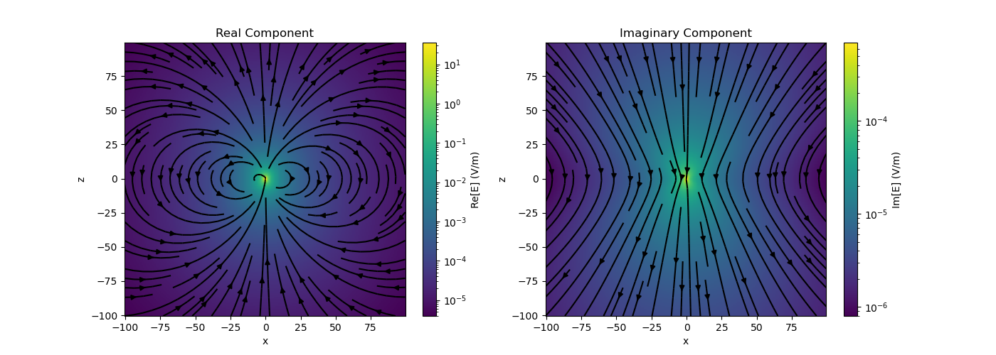
Electric Field from a Harmonic Electric Current Dipole Source#
Here, we compute the electric fields for a harmonic electric current dipole source in the z direction. Based on the geometry of the problem, we expect electric fields in the x and z directions, but none in the y direction.
# Defining electric dipole location and frequency
source_location = np.r_[0, 0, 0]
frequency = 1e3

# Defining observation locations (avoid placing observation at source)
x = np.arange(-100.5, 100.5, step=1.0)
y = np.r_[0]
z = x
observation_locations = utils.ndgrid(x, y, z)

# Define wholespace conductivity
sig = 1e-2

# Predict the fields
Ex, Ey, Ez = ElectricDipoleWholeSpace(
    observation_locations,
    source_location,
    sig,
    frequency,
    moment=[0, 0, 1],
    fieldType="e",
    mu_r=1,
    eps_r=1,
)

# Plot
fig = plt.figure(figsize=(14, 5))

explt = Ex.reshape(x.size, z.size)
ezplt = Ez.reshape(x.size, z.size)

ax1 = fig.add_subplot(121)
absE = np.sqrt(Ex.real**2 + Ey.real**2 + Ez.real**2)
pc1 = ax1.pcolor(x, z, absE.reshape(x.size, z.size), norm=LogNorm())
ax1.streamplot(x, z, explt.real, ezplt.real, color="k", density=1)
ax1.set_xlim([x.min(), x.max()])
ax1.set_ylim([z.min(), z.max()])
ax1.set_title("Real Component")
ax1.set_xlabel("x")
ax1.set_ylabel("z")
cb1 = plt.colorbar(pc1, ax=ax1)
cb1.set_label("Re[E] (V/m)")

ax2 = fig.add_subplot(122)
absE = np.sqrt(Ex.imag**2 + Ey.imag**2 + Ez.imag**2)
pc2 = ax2.pcolor(x, z, absE.reshape(x.size, z.size), norm=LogNorm())
ax2.streamplot(x, z, explt.imag, ezplt.imag, color="k", density=1)
ax2.set_xlim([x.min(), x.max()])
ax2.set_ylim([z.min(), z.max()])
ax2.set_title("Imaginary Component")
ax2.set_xlabel("x")
ax2.set_ylabel("z")
cb2 = plt.colorbar(pc2, ax=ax2)
cb2.set_label("Im[E] (V/m)")
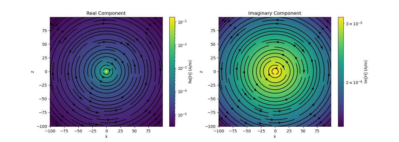
Magnetic Field from a Harmonic Electric Dipole Source#
Here, we compute the magnetic fields for a harmonic electric current dipole source in the y direction. Based on the geometry of the problem, we expect rotational magnetic fields in the x and z directions, but no fields in the y direction.
# Defining electric dipole location and frequency
source_location = np.r_[0, 0, 0]
frequency = 1e3

# Defining observation locations (avoid placing observation at source)
x = np.arange(-100.5, 100.5, step=1.0)
y = np.r_[0]
z = x
observation_locations = utils.ndgrid(x, y, z)

# Define wholespace conductivity
sig = 1e-2

# Predict the fields
Hx, Hy, Hz = ElectricDipoleWholeSpace(
    observation_locations,
    source_location,
    sig,
    frequency,
    moment=[0, 1, 0],
    fieldType="h",
    mu_r=1,
    eps_r=1,
)

# Plot
fig = plt.figure(figsize=(14, 5))

hxplt = Hx.reshape(x.size, z.size)
hzplt = Hz.reshape(x.size, z.size)

ax1 = fig.add_subplot(121)
absH = np.sqrt(Hx.real**2 + Hy.real**2 + Hz.real**2)
pc1 = ax1.pcolor(x, z, absH.reshape(x.size, z.size), norm=LogNorm())
ax1.streamplot(x, z, hxplt.real, hzplt.real, color="k", density=1)
ax1.set_xlim([x.min(), x.max()])
ax1.set_ylim([z.min(), z.max()])
ax1.set_title("Real Component")
ax1.set_xlabel("x")
ax1.set_ylabel("z")
cb1 = plt.colorbar(pc1, ax=ax1)
cb1.set_label("Re[H] (A/m)")

ax2 = fig.add_subplot(122)
absH = np.sqrt(Hx.imag**2 + Hy.imag**2 + Hz.imag**2)
pc2 = ax2.pcolor(x, z, absH.reshape(x.size, z.size), norm=LogNorm())
ax2.streamplot(x, z, hxplt.imag, hzplt.imag, color="k", density=1)
ax2.set_xlim([x.min(), x.max()])
ax2.set_ylim([z.min(), z.max()])
ax2.set_title("Imaginary Component")
ax2.set_xlabel("x")
ax2.set_ylabel("z")
cb2 = plt.colorbar(pc2, ax=ax2)
cb2.set_label("Im[H] (A/m)")
Total running time of the script: (0 minutes 13.043 seconds)
Estimated memory usage: 118 MB