Cylindrical Meshes

Cylindrical meshes are useful when the geological problem demonstrates rotational symmetry. In this case, we need only define how the model changes as a funcion of the radial distance and elevation; thus limiting the number of model parameters. Here we demonstrate various ways that models can be defined and mapped to cylindrical meshes. Some things we consider are:

• Adding structures of various shape to the model

• Parameterized models

• Models with 2 or more physical properties

Import modules

from discretize import CylindricalMesh
from SimPEG.utils import mkvc
from SimPEG import maps
import numpy as np
import matplotlib.pyplot as plt

Defining the mesh

Here, we create the tensor mesh that will be used for all examples.

def make_example_mesh():
    ncr = 20  # number of mesh cells in r
    ncz = 20  # number of mesh cells in z
    dh = 5.0  # cell width

    hr = [(dh, ncr), (dh, 5, 1.3)]
    hz = [(dh, 5, -1.3), (dh, ncz), (dh, 5, 1.3)]

    # Use flag of 1 to denote perfect rotational symmetry
    mesh = CylindricalMesh([hr, 1, hz], "0CC")

    return mesh

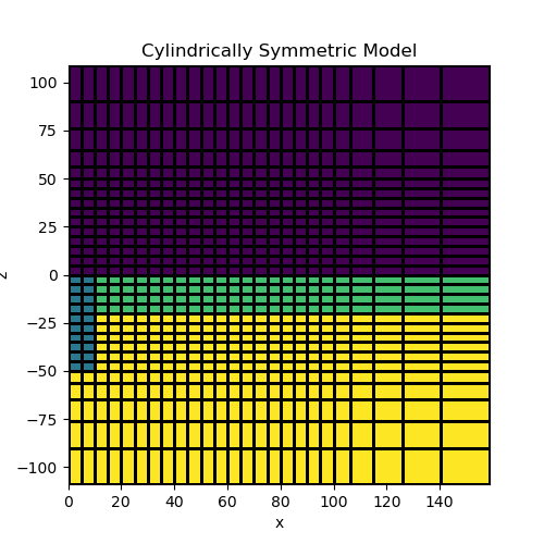
Vertical Pipe and a 2 Layered Earth

In this example we create a model containing a vertical pipe and a layered Earth. We will see that we need only define the model as a function of r and z. Models of this type are plotted from the center of the mesh to the total radial distance of the mesh. That is why pipes and rings look like blocks.

mesh = make_example_mesh()

background_value = 100.0
layer_value = 70.0
pipe_value = 40.0

# Find cells below topography and define mapping
air_value = 0.0
ind_active = mesh.gridCC[:, 2] < 0.0
model_map = maps.InjectActiveCells(mesh, ind_active, air_value)

# Define the model
model = background_value * np.ones(ind_active.sum())
ind_layer = (mesh.gridCC[ind_active, 2] > -20.0) & (mesh.gridCC[ind_active, 2] < -0)
model[ind_layer] = layer_value
ind_pipe = (
    (mesh.gridCC[ind_active, 0] < 10.0)
    & (mesh.gridCC[ind_active, 2] > -50.0)
    & (mesh.gridCC[ind_active, 2] < 0.0)
)
model[ind_pipe] = pipe_value


# Plotting
fig = plt.figure(figsize=(5, 5))
ax = fig.add_subplot(111)
mesh.plot_image(model_map * model, ax=ax, grid=True)
ax.set_title("Cylindrically Symmetric Model")

Text(0.5, 1.0, 'Cylindrically Symmetric Model')

Combo Maps

Here we demonstrate how combo maps can be used to create a single mapping from the model to the mesh. In this case, our model consists of log-conductivity values but we want to plot the resistivity. To accomplish this we must take the exponent of our model values, then take the reciprocal, then map from below surface cell to the mesh.

mesh = make_example_mesh()

background_value = np.log(1.0 / 100.0)
layer_value = np.log(1.0 / 70.0)
pipe_value = np.log(1.0 / 40.0)


# Find cells below topography and define mapping
air_value = 0.0
ind_active = mesh.gridCC[:, 2] < 0.0
active_map = maps.InjectActiveCells(mesh, ind_active, air_value)

# Define the model
model = background_value * np.ones(ind_active.sum())
ind_layer = (mesh.gridCC[ind_active, 2] > -20.0) & (mesh.gridCC[ind_active, 2] < -0)
model[ind_layer] = layer_value
ind_pipe = (
    (mesh.gridCC[ind_active, 0] < 10.0)
    & (mesh.gridCC[ind_active, 2] > -50.0)
    & (mesh.gridCC[ind_active, 2] < 0.0)
)
model[ind_pipe] = pipe_value

# Define a single mapping from model to mesh
exponential_map = maps.ExpMap()
reciprocal_map = maps.ReciprocalMap()
model_map = active_map * reciprocal_map * exponential_map

# Plotting
fig = plt.figure(figsize=(5, 5))
ax = fig.add_subplot(111)
mesh.plot_image(model_map * model, ax=ax, grid=True)
ax.set_title("Cylindrically Symmetric Model")

Text(0.5, 1.0, 'Cylindrically Symmetric Model')

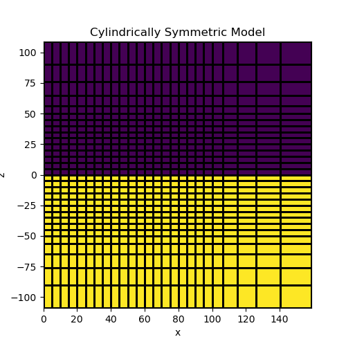
Parameterized pipe model

Instead of defining a model value for each sub-surface cell, we can define the model in terms of a small number of parameters. Here we parameterize the model as a block in a half-space. We then create a mapping which projects this model onto the mesh.

mesh = make_example_mesh()

background_value = 100.0  # background value
pipe_value = 40.0  # pipe value
rc, zc = 0.0, -25.0  # center of pipe
dr, dz = 20.0, 50.0  # dimensions in r, z

# Find cells below topography and define mapping
air_value = 0.0
ind_active = mesh.gridCC[:, 2] < 0.0
active_map = maps.InjectActiveCells(mesh, ind_active, air_value)

# Define the model on subsurface cells
model = np.r_[
    background_value, pipe_value, rc, dr, 0.0, 1.0, zc, dz
]  # add dummy values for phi
parametric_map = maps.ParametricBlock(mesh, indActive=ind_active, epsilon=1e-10, p=8.0)

# Define a single mapping from model to mesh
model_map = active_map * parametric_map

# Plotting
fig = plt.figure(figsize=(5, 5))
ax = fig.add_subplot(111)
mesh.plot_image(model_map * model, ax=ax, grid=True)
ax.set_title("Cylindrically Symmetric Model")

Text(0.5, 1.0, 'Cylindrically Symmetric Model')

Using Wire Maps

Wire maps are needed when the model is comprised of two or more parameter types (e.g. conductivity and magnetic permeability). Because the model vector contains all values for all parameter types, we need to use “wires” to extract the values for a particular parameter type.

Here we will define a model consisting of log-conductivity values and magnetic permeability values. We wish to plot the conductivity and permeability on the mesh. Wires are used to keep track of the mapping between the model vector and a particular physical property type.

mesh = make_example_mesh()

background_sigma = np.log(100.0)
layer_sigma = np.log(70.0)
pipe_sigma = np.log(40.0)
background_mu = 1.0
pipe_mu = 5.0

# Find cells below topography and define mapping
air_value = 0.0
ind_active = mesh.gridCC[:, 2] < 0.0
active_map = maps.InjectActiveCells(mesh, ind_active, air_value)

# Define model for cells under the surface topography
N = int(ind_active.sum())
model = np.kron(np.ones((N, 1)), np.c_[background_sigma, background_mu])

# Add a conductive and non-permeable layer
ind_layer = (mesh.gridCC[ind_active, 2] > -20.0) & (mesh.gridCC[ind_active, 2] < -0)
model[ind_layer, 0] = layer_sigma

# Add a conductive and permeable pipe
ind_pipe = (
    (mesh.gridCC[ind_active, 0] < 10.0)
    & (mesh.gridCC[ind_active, 2] > -50.0)
    & (mesh.gridCC[ind_active, 2] < 0.0)
)
model[ind_pipe] = np.c_[pipe_sigma, pipe_mu]

# Create model vector and wires
model = mkvc(model)
wire_map = maps.Wires(("log_sigma", N), ("mu", N))

# Use combo maps to map from model to mesh
sigma_map = active_map * maps.ExpMap() * wire_map.log_sigma
mu_map = active_map * wire_map.mu

# Plotting
fig = plt.figure(figsize=(5, 5))
ax = fig.add_subplot(111)
mesh.plot_image(sigma_map * model, ax=ax, grid=True)
ax.set_title("Cylindrically Symmetric Model")

Text(0.5, 1.0, 'Cylindrically Symmetric Model')

Estimated memory usage: 8 MB