Forward Simulation of Gradiometry Data for Magnetic Vector Models

Here we use the module SimPEG.potential_fields.magnetics to predict magnetic gradiometry data for magnetic vector models. The simulation is performed on a Tree mesh. For this tutorial, we focus on the following:

• How to define the survey when we want to measured multiple field components

• How to predict magnetic data in the case of remanence

• How to include surface topography

• How to construct tree meshes based on topography and survey geometry

• The units of the physical property model and resulting data

Import Modules

import numpy as np
from scipy.interpolate import LinearNDInterpolator
import matplotlib as mpl
import matplotlib.pyplot as plt

from discretize import TreeMesh
from discretize.utils import mkvc, refine_tree_xyz, active_from_xyz
from SimPEG.utils import plot2Ddata, model_builder, mat_utils
from SimPEG import maps
from SimPEG.potential_fields import magnetics

# sphinx_gallery_thumbnail_number = 2

Topography

Here we define surface topography as an (N, 3) numpy array. Topography could also be loaded from a file.

[x_topo, y_topo] = np.meshgrid(np.linspace(-200, 200, 41), np.linspace(-200, 200, 41))
z_topo = -15 * np.exp(-(x_topo**2 + y_topo**2) / 80**2)
x_topo, y_topo, z_topo = mkvc(x_topo), mkvc(y_topo), mkvc(z_topo)
xyz_topo = np.c_[x_topo, y_topo, z_topo]

Defining the Survey

Here, we define survey that will be used for the simulation. Magnetic surveys are simple to create. The user only needs an (N, 3) array to define the xyz locations of the observation locations, the list of field components which are to be modeled and the properties of the Earth’s field.

# Define the observation locations as an (N, 3) numpy array or load them.
x = np.linspace(-80.0, 80.0, 17)
y = np.linspace(-80.0, 80.0, 17)
x, y = np.meshgrid(x, y)
x, y = mkvc(x.T), mkvc(y.T)
fun_interp = LinearNDInterpolator(np.c_[x_topo, y_topo], z_topo)
z = fun_interp(np.c_[x, y]) + 10  # Flight height 10 m above surface.
receiver_locations = np.c_[x, y, z]

# Define the component(s) of the field we want to simulate as strings within
# a list. Here we measure the x, y and z derivatives of the Bz anomaly at
# each observation location.
components = ["bxz", "byz", "bzz"]

# Use the observation locations and components to define the receivers. To
# simulate data, the receivers must be defined as a list.
receiver_list = magnetics.receivers.Point(receiver_locations, components=components)

receiver_list = [receiver_list]

# Define the inducing field H0 = (intensity [nT], inclination [deg], declination [deg])
field_inclination = 60
field_declination = 30
field_strength = 50000

source_field = magnetics.sources.UniformBackgroundField(
    receiver_list=receiver_list,
    amplitude=field_strength,
    inclination=field_inclination,
    declination=field_declination,
)

# Define the survey
survey = magnetics.survey.Survey(source_field)

Defining an OcTree Mesh

Here, we create the OcTree mesh that will be used to predict magnetic gradiometry data for the forward simuulation.

dx = 5  # minimum cell width (base mesh cell width) in x
dy = 5  # minimum cell width (base mesh cell width) in y
dz = 5  # minimum cell width (base mesh cell width) in z

x_length = 240.0  # domain width in x
y_length = 240.0  # domain width in y
z_length = 120.0  # domain width in y

# Compute number of base mesh cells required in x and y
nbcx = 2 ** int(np.round(np.log(x_length / dx) / np.log(2.0)))
nbcy = 2 ** int(np.round(np.log(y_length / dy) / np.log(2.0)))
nbcz = 2 ** int(np.round(np.log(z_length / dz) / np.log(2.0)))

# Define the base mesh
hx = [(dx, nbcx)]
hy = [(dy, nbcy)]
hz = [(dz, nbcz)]
mesh = TreeMesh([hx, hy, hz], x0="CCN")

# Refine based on surface topography
mesh = refine_tree_xyz(
    mesh, xyz_topo, octree_levels=[2, 2], method="surface", finalize=False
)

# Refine box base on region of interest
xp, yp, zp = np.meshgrid([-100.0, 100.0], [-100.0, 100.0], [-80.0, 0.0])
xyz = np.c_[mkvc(xp), mkvc(yp), mkvc(zp)]

mesh = refine_tree_xyz(mesh, xyz, octree_levels=[2, 2], method="box", finalize=False)

mesh.finalize()

/home/vsts/work/1/s/tutorials/04-magnetics/plot_2b_magnetics_mvi.py:124: DeprecationWarning:

The surface option is deprecated as of `0.9.0` please update your code to use the `TreeMesh.refine_surface` functionality. It will be removed in a future version of discretize.

/home/vsts/work/1/s/tutorials/04-magnetics/plot_2b_magnetics_mvi.py:132: DeprecationWarning:

The box option is deprecated as of `0.9.0` please update your code to use the `TreeMesh.refine_bounding_box` functionality. It will be removed in a future version of discretize.

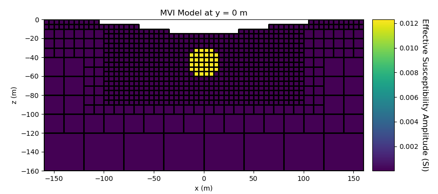
Create Magnetic Vector Intensity Model (MVI)

Magnetic vector models are defined by three-component effective susceptibilities. To create a magnetic vector model, we must

1) Define the magnetic susceptibility for each cell. Then multiply by the unit vector direction of the inducing field. (induced contribution) 2) Define the remanent magnetization vector for each cell and normalize by the magnitude of the Earth’s field (remanent contribution) 3) Sum the induced and remanent contributions 4) Define as a vector np.r_[chi_1, chi_2, chi_3]

# Define susceptibility values for each unit in SI
background_susceptibility = 0.0001
sphere_susceptibility = 0.01

# Find cells active in the forward modeling (cells below surface)
ind_active = active_from_xyz(mesh, xyz_topo)

# Define mapping from model to active cells
nC = int(ind_active.sum())
model_map = maps.IdentityMap(nP=3 * nC)  # model has 3 parameters for each cell

# Define susceptibility for each cell
susceptibility_model = background_susceptibility * np.ones(ind_active.sum())
ind_sphere = model_builder.get_indices_sphere(np.r_[0.0, 0.0, -45.0], 15.0, mesh.gridCC)
ind_sphere = ind_sphere[ind_active]
susceptibility_model[ind_sphere] = sphere_susceptibility

# Compute the unit direction of the inducing field in Cartesian coordinates
field_direction = mat_utils.dip_azimuth2cartesian(field_inclination, field_declination)

# Multiply susceptibility model to obtain the x, y, z components of the
# effective susceptibility contribution from induced magnetization.
susceptibility_model = np.outer(susceptibility_model, field_direction)

# Define the effective susceptibility contribution for remanent magnetization to have a
# magnitude of 0.006 SI, with inclination -45 and declination 90
remanence_inclination = -45.0
remanence_declination = 90.0
remanence_susceptibility = 0.01

remanence_model = np.zeros(np.shape(susceptibility_model))
effective_susceptibility_sphere = (
    remanence_susceptibility
    * mat_utils.dip_azimuth2cartesian(remanence_inclination, remanence_declination)
)
remanence_model[ind_sphere, :] = effective_susceptibility_sphere

# Define effective susceptibility model as a vector np.r_[chi_x, chi_y, chi_z]
plotting_model = susceptibility_model + remanence_model
model = mkvc(plotting_model)

# Plot Effective Susceptibility Model
fig = plt.figure(figsize=(9, 4))

plotting_map = maps.InjectActiveCells(mesh, ind_active, np.nan)
plotting_model = np.sqrt(np.sum(plotting_model, axis=1) ** 2)
ax1 = fig.add_axes([0.1, 0.12, 0.73, 0.78])
mesh.plot_slice(
    plotting_map * plotting_model,
    normal="Y",
    ax=ax1,
    ind=int(mesh.h[1].size / 2),
    grid=True,
    clim=(np.min(plotting_model), np.max(plotting_model)),
)
ax1.set_title("MVI Model at y = 0 m")
ax1.set_xlabel("x (m)")
ax1.set_ylabel("z (m)")

ax2 = fig.add_axes([0.85, 0.12, 0.05, 0.78])
norm = mpl.colors.Normalize(vmin=np.min(plotting_model), vmax=np.max(plotting_model))
cbar = mpl.colorbar.ColorbarBase(ax2, norm=norm, orientation="vertical")
cbar.set_label(
    "Effective Susceptibility Amplitude (SI)", rotation=270, labelpad=15, size=12
)

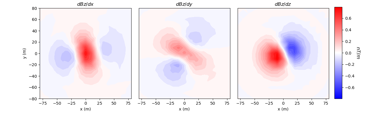
Simulation: Gradiometry Data for an MVI Model

Here we predict magnetic gradiometry data for an effective susceptibility model in the case of remanent magnetization.

# Define the forward simulation. By setting the 'store_sensitivities' keyword
# argument to "forward_only", we simulate the data without storing the sensitivities
simulation = magnetics.simulation.Simulation3DIntegral(
    survey=survey,
    mesh=mesh,
    chiMap=model_map,
    ind_active=ind_active,
    model_type="vector",
    store_sensitivities="forward_only",
)

# Compute predicted data for some model
dpred = simulation.dpred(model)
n_data = len(dpred)

# Plot
fig = plt.figure(figsize=(13, 4))
v_max = np.max(np.abs(dpred))

ax1 = fig.add_axes([0.1, 0.15, 0.25, 0.78])
plot2Ddata(
    receiver_list[0].locations,
    dpred[0:n_data:3],
    ax=ax1,
    ncontour=30,
    clim=(-v_max, v_max),
    contourOpts={"cmap": "bwr"},
)
ax1.set_title("$dBz/dx$")
ax1.set_xlabel("x (m)")
ax1.set_ylabel("y (m)")

ax2 = fig.add_axes([0.36, 0.15, 0.25, 0.78])
cplot2 = plot2Ddata(
    receiver_list[0].locations,
    dpred[1:n_data:3],
    ax=ax2,
    ncontour=30,
    clim=(-v_max, v_max),
    contourOpts={"cmap": "bwr"},
)
cplot2[0].set_clim((-v_max, v_max))
ax2.set_title("$dBz/dy$")
ax2.set_xlabel("x (m)")
ax2.set_yticks([])

ax3 = fig.add_axes([0.62, 0.15, 0.25, 0.78])
cplot3 = plot2Ddata(
    receiver_list[0].locations,
    dpred[2:n_data:3],
    ax=ax3,
    ncontour=30,
    clim=(-v_max, v_max),
    contourOpts={"cmap": "bwr"},
)
cplot3[0].set_clim((-v_max, v_max))
ax3.set_title("$dBz/dz$")
ax3.set_xlabel("x (m)")
ax3.set_yticks([])

ax4 = fig.add_axes([0.88, 0.15, 0.02, 0.79])
norm = mpl.colors.Normalize(vmin=-v_max, vmax=v_max)
cbar = mpl.colorbar.ColorbarBase(
    ax4, norm=norm, orientation="vertical", cmap=mpl.cm.bwr
)
cbar.set_label("$nT/m$", rotation=270, labelpad=15, size=12)

plt.show()

Estimated memory usage: 8 MB