1D Forward Simulation for a Susceptible and Chargeable Earth

Here we use the module simpeg.electromangetics.frequency_domain_1d to compare predicted frequency domain data for a single sounding when the Earth is purely conductive, conductive and magnetically susceptible, and when it is chargeable. In this tutorial, we focus on:

• Defining receivers, sources and the survey

• Defining physical properties when the Earth is chargeable and/or magnetically susceptibility

• Setting physical property values as constant in the simulation

Our survey geometry consists of a vertical magnetic dipole source located 30 m above the Earth’s surface. The receiver is offset 10 m horizontally from the source.

Import Modules

import numpy as np
from matplotlib import pyplot as plt

from simpeg import maps
import simpeg.electromagnetics.frequency_domain as fdem
from simpeg.electromagnetics.utils.em1d_utils import ColeCole

plt.rcParams.update({"font.size": 16})

# sphinx_gallery_thumbnail_number = 2

Create Survey

Here we demonstrate a general way to define the receivers, sources and survey. For this tutorial, the source is a vertical magnetic dipole that will be used to simulate data at a number of frequencies. The receivers measure real and imaginary ppm data.

# Frequencies being observed in Hz
frequencies = np.logspace(0, 8, 41)

# Define a list of receivers. The real and imaginary components are defined
# as separate receivers.
receiver_location = np.array([10.0, 0.0, 10.0])
receiver_orientation = "z"  # "x", "y" or "z"
data_type = "ppm"  # "secondary", "total" or "ppm"

receiver_list = [
    fdem.receivers.PointMagneticFieldSecondary(
        receiver_location,
        orientation=receiver_orientation,
        data_type=data_type,
        component="both",
    )
]

# Define a source list. A source must defined for each frequency.
source_location = np.array([0.0, 0.0, 10.0])
source_orientation = "z"  # "x", "y" or "z"
moment = 1.0  # dipole moment

source_list = []
for freq in frequencies:
    source_list.append(
        fdem.sources.MagDipole(
            receiver_list=receiver_list,
            frequency=freq,
            location=source_location,
            orientation=source_orientation,
            moment=moment,
        )
    )


# Define a 1D FDEM survey
survey = fdem.survey.Survey(source_list)

Defining a Layered Earth Model

Here, we define the layer thicknesses and physical properties for our 1D simulation. If we have N layers, parameters for the physical properties must be defined for each layer and we must provide N-1 layer thicknesses. The lowest layer is assumed to extend to infinity.

For this tutorial, we predict the response for a halfspace model, however the script has been generalized to work for an arbitrary number of layers. If the Earth is a halfspace, the thicknesses could instead be defined by an empty array, and each physical property value by an array of length 1.

# Layer thicknesses
thicknesses = np.array([20, 40])
n_layer = len(thicknesses) + 1

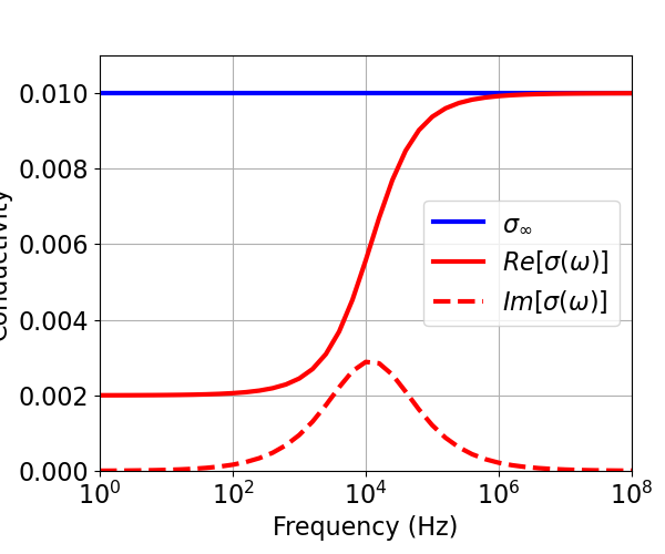
# In SimPEG, the Cole-Cole model is used to define a frequency-dependent
# electrical conductivity when the Earth is chargeable.
sigma = 1e-2  # infinite conductivity in S/m
eta = 0.8  # intrinsice chargeability [0, 1]
tau = 0.0001  # central time-relaxation constant in seconds
c = 0.8  # phase constant [0, 1]

# Magnetic susceptibility in SI
chi = 0.2

# For each physical property, the parameters must be defined for each layer.
# In this case, we must define all parameters for the Cole-Cole conductivity
# as well as the magnetic susceptibility.
sigma_model = sigma * np.ones(n_layer)
eta_model = eta * np.ones(n_layer)
tau_model = tau * np.ones(n_layer)
c_model = c * np.ones(n_layer)
mu0 = 4 * np.pi * 1e-7
mu_model = mu0 * (1 + chi) * np.ones(n_layer)

# Here, we let the infinite conductivity be the model. As a result, we only
# need to define the mapping for this parameter. All other parameters used
# to define physical properties will be fixed when creating the simulation.
model_mapping = maps.IdentityMap(nP=n_layer)

# Plot complex conductivity at all frequencies
sigma_complex = ColeCole(frequencies, sigma, eta, tau, c)

fig = plt.figure(figsize=(6, 5))
ax = fig.add_axes([0.15, 0.15, 0.8, 0.75])
ax.semilogx(frequencies, sigma * np.ones(len(frequencies)), "b", lw=3)
ax.semilogx(frequencies, np.real(sigma_complex), "r", lw=3)
ax.semilogx(frequencies, np.imag(sigma_complex), "r--", lw=3)
ax.grid()
ax.set_xlim(np.min(frequencies), np.max(frequencies))
ax.set_ylim(0.0, 1.1 * sigma)
ax.set_xlabel("Frequency (Hz)")
ax.set_ylabel("Conductivity")
ax.legend(
    [r"$\sigma_{\infty}$", r"$Re[\sigma (\omega)]$", r"$Im[\sigma (\omega)]$"],
    loc="center right",
)
plt.show()

Define the Forward Simulation and Predict Data

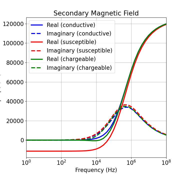
Here we predict the FDEM sounding for several halfspace models (conductive, susceptible, chargeable). Since the physical properties defining the Earth are different, it requires a separate simulation object be created for each case. Each simulation requires the user define the survey, the layer thicknesses and a mapping.

A universal mapping was created by letting sigma be the model. All other parameters used to define the physical properties are permanently set when defining the simulation.

When using the simpeg.electromagnetics.frequency_domain_1d module, note that predicted data are organized by source, then by receiver, then by frequency.

# Response for conductive Earth
simulation = fdem.Simulation1DLayered(
    survey=survey, thicknesses=thicknesses, sigmaMap=model_mapping
)

dpred = simulation.dpred(sigma_model)

# Simulate response for a conductive and susceptible Earth
simulation_susceptible = fdem.Simulation1DLayered(
    survey=survey, thicknesses=thicknesses, sigmaMap=model_mapping, mu=mu_model
)

dpred_susceptible = simulation_susceptible.dpred(sigma_model)

# Simulate response for a chargeable Earth
simulation_chargeable = fdem.Simulation1DLayered(
    survey=survey,
    thicknesses=thicknesses,
    sigmaMap=model_mapping,
    eta=eta,
    tau=tau,
    c=c,
)

dpred_chargeable = simulation_chargeable.dpred(sigma_model)

Plotting Results

fig = plt.figure(figsize=(7, 7))
ax = fig.add_axes([0.15, 0.1, 0.8, 0.8])
ax.semilogx(frequencies, dpred[0::2], "b-", lw=3)
ax.semilogx(frequencies, dpred[1::2], "b--", lw=3)
ax.semilogx(frequencies, dpred_susceptible[0::2], "r-", lw=3)
ax.semilogx(frequencies, dpred_susceptible[1::2], "r--", lw=3)
ax.semilogx(frequencies, dpred_chargeable[0::2], "g-", lw=3)
ax.semilogx(frequencies, dpred_chargeable[1::2], "g--", lw=3)
ax.set_xlim([frequencies.min(), frequencies.max()])
ax.grid()
ax.set_xlabel("Frequency (Hz)")
ax.set_ylabel("|Hs| (A/m)")
ax.set_title("Secondary Magnetic Field")
ax.legend(
    (
        "Real (conductive)",
        "Imaginary (conductive)",
        "Real (susceptible)",
        "Imaginary (susceptible)",
        "Real (chargeable)",
        "Imaginary (chargeable)",
    )
)

<matplotlib.legend.Legend object at 0x7f6584405300>

Estimated memory usage: 293 MB