1D Forward Simulation with Chargeable and/or Magnetic Viscosity

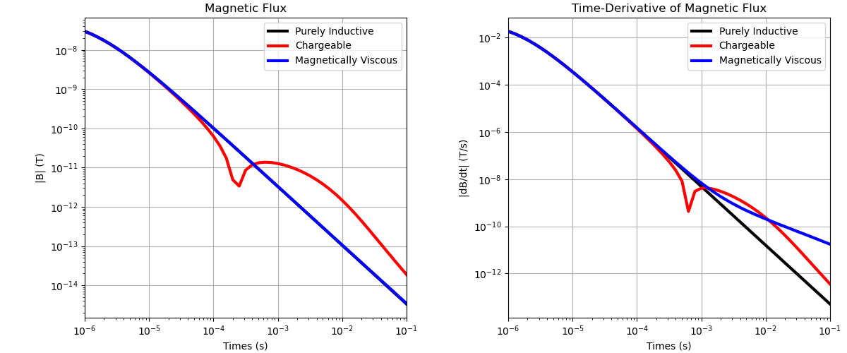
Here we use the module simpeg.electromangetics.time_domain_1d to compare predicted time domain data for a single sounding when the Earth is purely conductive, chargeable and/or magnetically viscous. In this tutorial, we focus on:

• Defining receivers, sources, waveform and the survey

• Defining physical properties when the Earth is chargeable and/or magnetically viscous

• Setting physical property values as constant in the simulation

Our survey geometry consists of a horizontal loop source with a radius of 10 m located 0.5 m above the Earth’s surface. The receiver is located at the centre of the loop and measures the vertical component of the response.

Import Modules

import numpy as np
from matplotlib import pyplot as plt

from simpeg import maps
import simpeg.electromagnetics.time_domain as tdem
from simpeg.electromagnetics.utils.em1d_utils import ColeCole, LogUniform

# sphinx_gallery_thumbnail_number = 3

Create Survey

Here we demonstrate a general way to define the receivers, sources, waveforms and survey. For this tutorial, the source is a horizontal loop whose current waveform is a unit step-off. Receivers are defined to measure the vertical component of the magnetic flux density and its time-derivative at the loop’s center.

source_location = np.array([0.0, 0.0, 0.5])
source_orientation = "z"  # "x", "y" or "z"
current_amplitude = 1.0  # maximum amplitude of source current
source_radius = 10.0  # loop radius

receiver_location = np.array([0.0, 0.0, 0.5])
receiver_orientation = "z"  # "x", "y" or "z"
times = np.logspace(-6, -1, 51)  # time channels (s)

# Receiver list
receiver_list = []
receiver_list.append(
    tdem.receivers.PointMagneticFluxDensity(
        receiver_location, times, orientation=receiver_orientation
    )
)
receiver_list.append(
    tdem.receivers.PointMagneticFluxTimeDerivative(
        receiver_location, times, orientation=receiver_orientation
    )
)

# Waveform
waveform = tdem.sources.StepOffWaveform()

# Sources
source_list = [
    tdem.sources.CircularLoop(
        receiver_list=receiver_list,
        location=source_location,
        waveform=waveform,
        current=current_amplitude,
        radius=source_radius,
    )
]

# Survey
survey = tdem.Survey(source_list)

Defining a 1D Layered Earth Model

Here, we define the layer thicknesses and physical properties for our 1D simulation. If we have N layers, parameters for the physical properties must be defined for each layer and we must provide N-1 layer thicknesses. The lowest layer is assumed to extend to infinity.

For this tutorial, we predict the response for a halfspace model, however the script has been generalized to work for an arbitrary number of layers. If the Earth is a halfspace, the thicknesses could instead be defined by an empty array, and each physical property value by an array of length 1.

# Layer thicknesses
thicknesses = np.array([40.0, 40.0])
n_layer = len(thicknesses) + 1

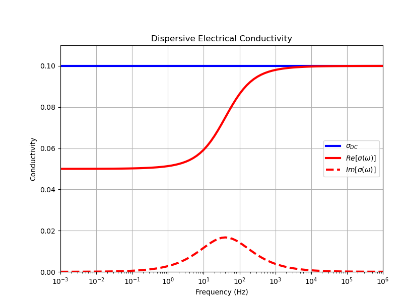
# In SimPEG, the Cole-Cole model is used to define a frequency-dependent
# electrical conductivity when the Earth is chargeable.
sigma = 1e-1  # infinite conductivity in S/m
eta = 0.5  # intrinsice chargeability [0, 1]
tau = 0.01  # central time-relaxation constant in seconds
c = 0.75  # phase constant [0, 1]

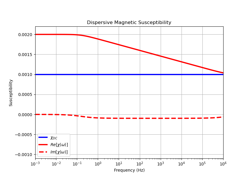
# In SimPEG, the a log-uniform distribution of time-relaxation constants is used
# to define a frequency-dependent susceptibility when the Earth exhibits
# magnetic viscosity
chi = 0.001  # infinite susceptibility in SI
dchi = 0.001  # amplitude of frequency-dependent susceptibility contribution
tau1 = 1e-7  # lower limit for time relaxation constants in seconds
tau2 = 1.0  # upper limit for time relaxation constants in seconds


# For each physical property, the parameters must be defined for each layer.
# In this case, we must define all parameters for the Cole-Cole conductivity
# as well as the frequency-dependent magnetic susceptibility.
sigma_model = sigma * np.ones(n_layer)
eta_model = eta * np.ones(n_layer)
tau_model = tau * np.ones(n_layer)
c_model = c * np.ones(n_layer)

chi_model = chi * np.ones(n_layer)
dchi_model = dchi * np.ones(n_layer)
tau1_model = tau1 * np.ones(n_layer)
tau2_model = tau2 * np.ones(n_layer)

# Here, we let the infinite conductivity be the model. As a result, we only
# need to define the mapping for this parameter. All other parameters used
# to define physical properties will be fixed when creating the simulation.
model_mapping = maps.IdentityMap(nP=n_layer)

# Compute and plot complex conductivity at all frequencies
frequencies = np.logspace(-3, 6, 91)
sigma_complex = ColeCole(frequencies, sigma, eta, tau, c)
chi_complex = LogUniform(frequencies, chi, dchi, tau1, tau2)

fig = plt.figure(figsize=(8, 6))
ax = fig.add_axes([0.15, 0.1, 0.8, 0.75])
ax.semilogx(frequencies, sigma * np.ones(len(frequencies)), "b", lw=3)
ax.semilogx(frequencies, np.real(sigma_complex), "r", lw=3)
ax.semilogx(frequencies, np.imag(sigma_complex), "r--", lw=3)
ax.grid()
ax.set_xlim(np.min(frequencies), np.max(frequencies))
ax.set_ylim(0.0, 1.1 * sigma)
ax.set_xlabel("Frequency (Hz)")
ax.set_ylabel("Conductivity")
ax.set_title("Dispersive Electrical Conductivity")
ax.legend(
    [r"$\sigma_{DC}$", r"$Re[\sigma (\omega)]$", r"$Im[\sigma (\omega)]$"],
    loc="center right",
)

fig = plt.figure(figsize=(8, 6))
ax = fig.add_axes([0.15, 0.1, 0.8, 0.75])
ax.semilogx(frequencies, chi * np.ones(len(frequencies)), "b", lw=3)
ax.semilogx(frequencies, np.real(chi_complex), "r", lw=3)
ax.semilogx(frequencies, np.imag(chi_complex), "r--", lw=3)
ax.grid()
ax.set_xlim(np.min(frequencies), np.max(frequencies))
ax.set_ylim(-1.1 * chi, 1.1 * (chi + dchi))
ax.set_xlabel("Frequency (Hz)")
ax.set_ylabel("Susceptibility")
ax.set_title("Dispersive Magnetic Susceptibility")
ax.legend(
    [r"$\chi_{DC}$", r"$Re[\chi (\omega)]$", r"$Im[\chi (\omega)]$"], loc="lower left"
)

• 
• 

<matplotlib.legend.Legend object at 0x7f3440b01d60>

Define the Forward Simulation and Predict Data

Here we predict the TDEM sounding for several halfspace models (conductive, chargeable, magnetically viscous). Since the physical properties defining the Earth are different, it requires a separate simulation object be created for each case. Each simulation requires the user define the survey, the layer thicknesses and a mapping.

A universal mapping was created by letting sigma be the model. All other parameters used to define the physical properties are permanently set when defining the simulation.

When using the simpeg.electromagnetics.time_domain_1d module, note that predicted data are organized by source, then by receiver, then by time channel.

# Simulate response for static conductivity
simulation_conductive = tdem.Simulation1DLayered(
    survey=survey, thicknesses=thicknesses, sigmaMap=model_mapping
)

dpred_conductive = simulation_conductive.dpred(sigma_model)

# Simulate response for a chargeable Earth
simulation_chargeable = tdem.Simulation1DLayered(
    survey=survey,
    thicknesses=thicknesses,
    sigmaMap=model_mapping,
    eta=eta,
    tau=tau,
    c=c,
)

dpred_chargeable = simulation_chargeable.dpred(sigma_model)

# Simulate response for viscous remanent magnetization
mu0 = 4 * np.pi * 1e-7
mu = mu0 * (1 + chi)
simulation_vrm = tdem.Simulation1DLayered(
    survey=survey,
    thicknesses=thicknesses,
    sigmaMap=model_mapping,
    mu=mu,
    dchi=dchi,
    tau1=tau1,
    tau2=tau2,
)

dpred_vrm = simulation_vrm.dpred(sigma_model)

/usr/share/miniconda/envs/simpeg-test/lib/python3.8/site-packages/numpy/core/_asarray.py:130: ComplexWarning:

Casting complex values to real discards the imaginary part

Plotting Results

fig = plt.figure(figsize=(12, 5))
ax1 = fig.add_axes([0.1, 0.1, 0.38, 0.85])
ax1.loglog(times, np.abs(dpred_conductive[0 : len(times)]), "k", lw=3)
ax1.loglog(times, np.abs(dpred_chargeable[0 : len(times)]), "r", lw=3)
ax1.loglog(times, np.abs(dpred_vrm[0 : len(times)]), "b", lw=3)
ax1.set_xlim([times.min(), times.max()])
ax1.grid()
ax1.legend(["Purely Inductive", "Chargeable", "Magnetically Viscous"])
ax1.set_xlabel("Times (s)")
ax1.set_ylabel("|B| (T)")
ax1.set_title("Magnetic Flux")

ax2 = fig.add_axes([0.6, 0.1, 0.38, 0.85])
ax2.loglog(times, np.abs(dpred_conductive[len(times) :]), "k", lw=3)
ax2.loglog(times, np.abs(dpred_chargeable[len(times) :]), "r", lw=3)
ax2.loglog(times, np.abs(dpred_vrm[len(times) :]), "b", lw=3)
ax2.set_xlim([times.min(), times.max()])
ax2.grid()
ax2.legend(["Purely Inductive", "Chargeable", "Magnetically Viscous"])
ax2.set_xlabel("Times (s)")
ax2.set_ylabel("|dB/dt| (T/s)")
ax2.set_title("Time-Derivative of Magnetic Flux")

Text(0.5, 1.0, 'Time-Derivative of Magnetic Flux')

Estimated memory usage: 9 MB