Note
Go to the end to download the full example code.
DC Resistivity Forward Simulation in 2.5D#
Here we use the module simpeg.electromagnetics.static.resistivity to predict DC resistivity data and plot using a pseudosection. In this tutorial, we focus on the following:
How to define the survey
How to define the forward simulation
How to predict normalized voltage data for a synthetic conductivity model
How to include surface topography
The units of the model and resulting data
Import modules#
from discretize import TreeMesh
from discretize.utils import mkvc, active_from_xyz

from simpeg.utils import model_builder
from simpeg.utils.io_utils.io_utils_electromagnetics import write_dcip2d_ubc
from simpeg import maps, data
from simpeg.electromagnetics.static import resistivity as dc
from simpeg.electromagnetics.static.utils.static_utils import (
    generate_dcip_sources_line,
    apparent_resistivity_from_voltage,
    plot_pseudosection,
)

import os
import numpy as np
import matplotlib as mpl
import matplotlib.pyplot as plt
from matplotlib.colors import LogNorm

try:
    from pymatsolver import Pardiso as Solver
except ImportError:
    from simpeg import SolverLU as Solver

write_output = False
mpl.rcParams.update({"font.size": 16})
# sphinx_gallery_thumbnail_number = 3
Defining Topography#
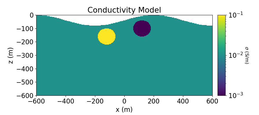
Here we define surface topography as an (N, 3) numpy array. Topography could also be loaded from a file. In our case, our survey takes place within a set of valleys that run North-South.
x_topo, y_topo = np.meshgrid(
    np.linspace(-3000, 3000, 601), np.linspace(-3000, 3000, 101)
)
z_topo = 40.0 * np.sin(2 * np.pi * x_topo / 800) - 40.0
x_topo, y_topo, z_topo = mkvc(x_topo), mkvc(y_topo), mkvc(z_topo)
topo_xyz = np.c_[x_topo, y_topo, z_topo]

# Create 2D topography. Since our 3D topography only changes in the x direction,
# it is easy to define the 2D topography projected along the survey line. For
# arbitrary topography and for an arbitrary survey orientation, the user must
# define the 2D topography along the survey line.
topo_2d = np.unique(topo_xyz[:, [0, 2]], axis=0)
Create Dipole-Dipole Survey#
Here we define a single EW survey line that uses a dipole-dipole configuration. For the source, we must define the AB electrode locations. For the receivers we must define the MN electrode locations. Instead of creating the survey from scratch (see 1D example), we will use the generat_dcip_survey_line utility.
# Define survey line parameters
survey_type = "dipole-dipole"
dimension_type = "2D"
data_type = "volt"
end_locations = np.r_[-400.0, 400.0]
station_separation = 40.0
num_rx_per_src = 10

# Generate source list for DC survey line
source_list = generate_dcip_sources_line(
    survey_type,
    data_type,
    dimension_type,
    end_locations,
    topo_2d,
    num_rx_per_src,
    station_separation,
)

# Define survey
survey = dc.survey.Survey(source_list)
Create Tree Mesh#
Here, we create the Tree mesh that will be used to predict DC data.
dh = 4  # base cell width
dom_width_x = 3200.0  # domain width x
dom_width_z = 2400.0  # domain width z
nbcx = 2 ** int(np.round(np.log(dom_width_x / dh) / np.log(2.0)))  # num. base cells x
nbcz = 2 ** int(np.round(np.log(dom_width_z / dh) / np.log(2.0)))  # num. base cells z

# Define the base mesh
hx = [(dh, nbcx)]
hz = [(dh, nbcz)]
mesh = TreeMesh([hx, hz], x0="CN")

# Mesh refinement based on topography
mesh.refine_surface(
    topo_xyz[:, [0, 2]],
    padding_cells_by_level=[0, 0, 4, 4],
    finalize=False,
)

# Mesh refinement near transmitters and receivers. First we need to obtain the
# set of unique electrode locations.
electrode_locations = np.c_[
    survey.locations_a,
    survey.locations_b,
    survey.locations_m,
    survey.locations_n,
]

unique_locations = np.unique(
    np.reshape(electrode_locations, (4 * survey.nD, 2)), axis=0
)

mesh.refine_points(unique_locations, padding_cells_by_level=[4, 4], finalize=False)

# Refine core mesh region
xp, zp = np.meshgrid([-600.0, 600.0], [-400.0, 0.0])
xyz = np.c_[mkvc(xp), mkvc(zp)]
mesh.refine_bounding_box(xyz, padding_cells_by_level=[0, 0, 2, 8], finalize=False)

mesh.finalize()
Create Conductivity Model and Mapping for Tree Mesh#
It is important that electrodes are not modeled as being in the air. Even if the electrodes are properly located along surface topography, they may lie above the discretized topography. This step is carried out to ensure all electrodes lie on the discretized surface.
# Define conductivity model in S/m (or resistivity model in Ohm m)
air_conductivity = 1e-8
background_conductivity = 1e-2
conductor_conductivity = 1e-1
resistor_conductivity = 1e-3

# Find active cells in forward modeling (cell below surface)
ind_active = active_from_xyz(mesh, topo_xyz[:, [0, 2]])

# Define mapping from model to active cells
nC = int(ind_active.sum())
conductivity_map = maps.InjectActiveCells(mesh, ind_active, air_conductivity)

# Define model
conductivity_model = background_conductivity * np.ones(nC)

ind_conductor = model_builder.get_indices_sphere(
    np.r_[-120.0, -160.0], 60.0, mesh.gridCC
)
ind_conductor = ind_conductor[ind_active]
conductivity_model[ind_conductor] = conductor_conductivity

ind_resistor = model_builder.get_indices_sphere(np.r_[120.0, -100.0], 60.0, mesh.gridCC)
ind_resistor = ind_resistor[ind_active]
conductivity_model[ind_resistor] = resistor_conductivity

# Plot Conductivity Model
fig = plt.figure(figsize=(9, 4))

plotting_map = maps.InjectActiveCells(mesh, ind_active, np.nan)
norm = LogNorm(vmin=1e-3, vmax=1e-1)

ax1 = fig.add_axes([0.14, 0.17, 0.68, 0.7])
mesh.plot_image(
    plotting_map * conductivity_model, ax=ax1, grid=False, pcolor_opts={"norm": norm}
)
ax1.set_xlim(-600, 600)
ax1.set_ylim(-600, 0)
ax1.set_title("Conductivity Model")
ax1.set_xlabel("x (m)")
ax1.set_ylabel("z (m)")

ax2 = fig.add_axes([0.84, 0.17, 0.03, 0.7])
cbar = mpl.colorbar.ColorbarBase(ax2, norm=norm, orientation="vertical")
cbar.set_label(r"$\sigma$ (S/m)", rotation=270, labelpad=15, size=12)

plt.show()

Project Survey to Discretized Topography#
It is important that electrodes are not model as being in the air. Even if the electrodes are properly located along surface topography, they may lie above the discretized topography. This step is carried out to ensure all electrodes like on the discretized surface.
survey.drape_electrodes_on_topography(mesh, ind_active, option="top")
Predict DC Resistivity Data#
Here we predict DC resistivity data. If the keyword argument sigmaMap is defined, the simulation will expect a conductivity model. If the keyword argument rhoMap is defined, the simulation will expect a resistivity model.
simulation = dc.simulation_2d.Simulation2DNodal(
    mesh, survey=survey, sigmaMap=conductivity_map, solver=Solver
)

# Predict the data by running the simulation. The data are the raw voltage in
# units of volts.
dpred = simulation.dpred(conductivity_model)
Plotting in Pseudo-Section#
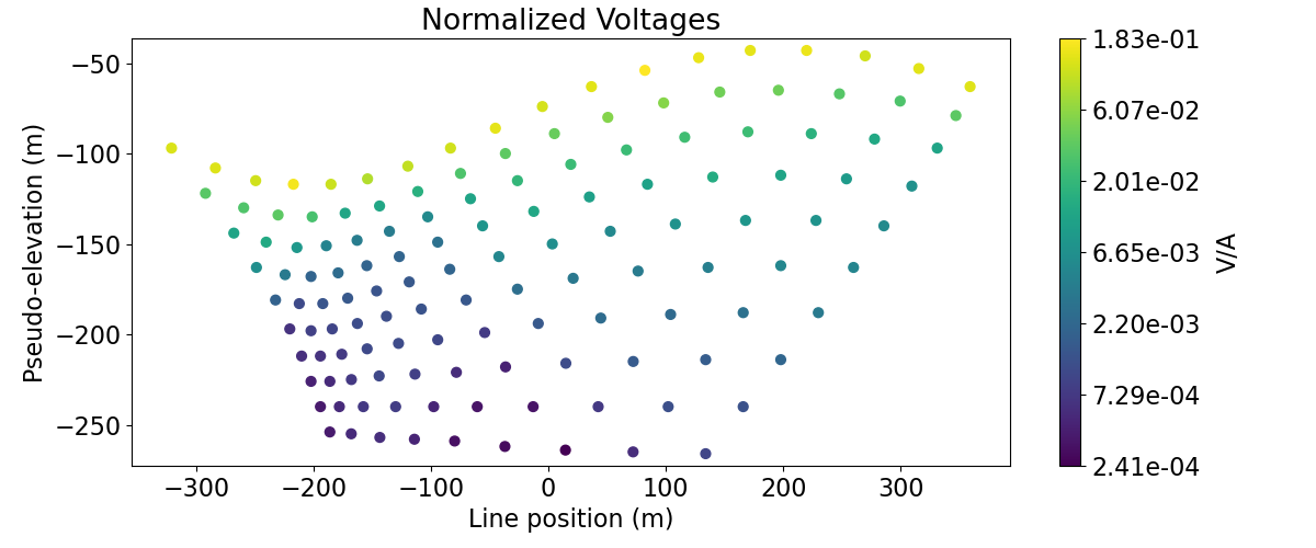
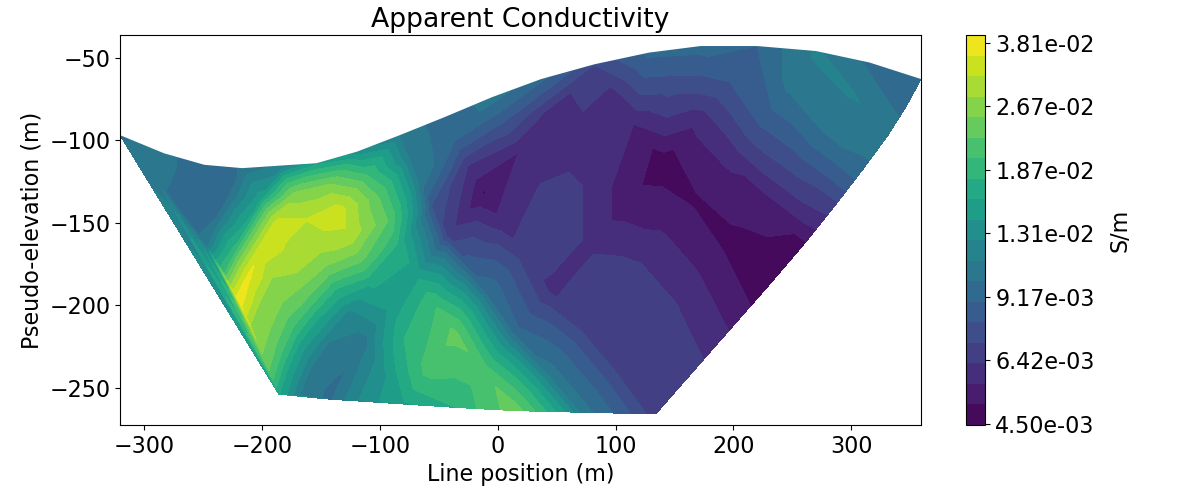
Here, we demonstrate how to plot 2D data in pseudo-section. First, we plot the voltages in pseudo-section as a scatter plot. This allows us to visualize the pseudo-sensitivity locations for our survey. Next, we plot the apparent conductivities in pseudo-section as a filled contour plot.
# Plot voltages pseudo-section
fig = plt.figure(figsize=(12, 5))
ax1 = fig.add_axes([0.1, 0.15, 0.75, 0.78])
plot_pseudosection(
    survey,
    dobs=np.abs(dpred),
    plot_type="scatter",
    ax=ax1,
    scale="log",
    cbar_label="V/A",
    scatter_opts={"cmap": mpl.cm.viridis},
)
ax1.set_title("Normalized Voltages")
plt.show()

# Get apparent conductivities from volts and survey geometry
apparent_conductivities = 1 / apparent_resistivity_from_voltage(survey, dpred)

# Plot apparent conductivity pseudo-section
fig = plt.figure(figsize=(12, 5))
ax1 = fig.add_axes([0.1, 0.15, 0.75, 0.78])
plot_pseudosection(
    survey,
    dobs=apparent_conductivities,
    plot_type="contourf",
    ax=ax1,
    scale="log",
    cbar_label="S/m",
    mask_topography=True,
    contourf_opts={"levels": 20, "cmap": mpl.cm.viridis},
)
ax1.set_title("Apparent Conductivity")
plt.show()
Optional: Write out dpred#
Write DC resistivity data, topography and true model
if write_output:
    dir_path = os.path.dirname(__file__).split(os.path.sep)
    dir_path.extend(["outputs"])
    dir_path = os.path.sep.join(dir_path) + os.path.sep

    if not os.path.exists(dir_path):
        os.mkdir(dir_path)

    # Add 10% Gaussian noise to each datum
    np.random.seed(225)
    std = 0.05 * np.abs(dpred)
    dc_noise = std * np.random.randn(len(dpred))
    dobs = dpred + dc_noise

    # Create a survey with the original electrode locations
    # and not the shifted ones
    # Generate source list for DC survey line
    source_list = generate_dcip_sources_line(
        survey_type,
        data_type,
        dimension_type,
        end_locations,
        topo_xyz,
        num_rx_per_src,
        station_separation,
    )
    survey_original = dc.survey.Survey(source_list)

    # Write out data at their original electrode locations (not shifted)
    data_obj = data.Data(survey_original, dobs=dobs, standard_deviation=std)
    fname = dir_path + "dc_data.obs"
    write_dcip2d_ubc(fname, data_obj, "volt", "dobs")

    fname = dir_path + "topo_xyz.txt"
    np.savetxt(fname, topo_xyz, fmt="%.4e")
Total running time of the script: (0 minutes 11.768 seconds)
Estimated memory usage: 164 MB

