Note
Go to the end to download the full example code.
Maps: ComboMaps#
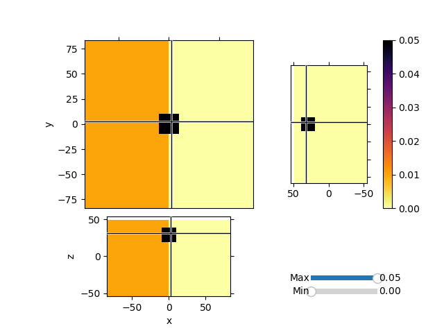
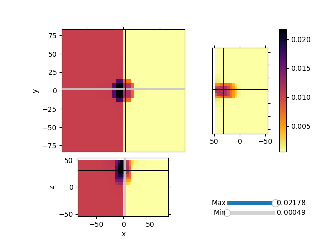
Invert synthetic magnetic data with variable background values and a single block anomaly buried at depth. We will use the Sum Map to invert for both the background values and an heterogeneous susceptibiilty model.
1
Running inversion with SimPEG v0.25.2.dev9+g43b0120dd
================================================= Projected GNCG =================================================
  #     beta     phi_d     phi_m       f      |proj(x-g)-x|  LS   iter_CG   CG |Ax-b|/|b|  CG |Ax-b|   Comment
-----------------------------------------------------------------------------------------------------------------
   0  5.52e+05  9.11e+06  4.27e-04  9.11e+06                         0           inf          inf
   1  5.52e+05  1.32e+05  7.72e-02  1.75e+05    6.29e+01      0      3        7.86e-04     1.08e+06
   2  2.76e+05  4.45e+04  2.40e-01  1.11e+05    3.53e+01      0      9        6.08e-04     2.70e+04
   3  1.38e+05  1.89e+04  3.69e-01  6.99e+04    4.92e+01      0      10       2.39e-02     3.47e+04
   4  6.90e+04  6.02e+03  4.81e-01  3.92e+04    5.53e+01      0      9        4.72e-04     5.02e+03
   5  3.45e+04  4.41e+03  5.15e-01  2.22e+04    4.76e+01      1      10       9.91e-03     4.95e+03
   6  1.73e+04  8.48e+02  6.04e-01  1.13e+04    3.56e+01      0      10       4.81e-04     5.20e+03
   7  8.63e+03  8.40e+02  6.05e-01  6.06e+03    4.85e+01      4      10       8.31e-02     1.23e+04
   8  4.31e+03  3.91e+02  6.48e-01  3.19e+03    5.30e+01      0      10       1.29e-01     1.48e+05
Reached starting chifact with l2-norm regularization: Start IRLS steps...
irls_threshold 0.010246853726920987
irls_threshold 0.011883120432964845
   9  4.31e+03  4.12e+02  8.57e-01  4.11e+03    2.63e+01      3      10       6.02e-02     1.65e+04
  10  4.31e+03  4.55e+02  8.94e-01  4.31e+03    3.55e+01      1      10       7.41e-03     1.33e+04
  11  3.51e+03  4.55e+02  9.64e-01  3.84e+03    6.02e+01     10      10       4.10e-02     8.55e+04
  12  2.86e+03  4.71e+02  9.73e-01  3.26e+03    6.02e+01      3      10       1.69e-01     3.53e+05
  13  2.29e+03  4.20e+02  9.76e-01  2.65e+03    3.35e+01      0      10       6.46e-02     7.63e+04
  14  2.29e+03  4.25e+02  1.02e+00  2.76e+03    4.49e+01      4      10       6.71e-01     9.49e+04
  15  2.29e+03  4.58e+02  9.68e-01  2.67e+03    5.78e+01      0      10       2.06e-02     1.46e+04
  16  1.86e+03  4.58e+02  9.68e-01  2.26e+03    3.56e+01      8      10       3.81e-02     6.95e+04
  17  1.51e+03  4.51e+02  9.08e-01  1.82e+03    3.56e+01      2      10       1.25e-02     2.29e+04
  18  1.23e+03  4.01e+02  8.62e-01  1.46e+03    5.88e+01      0      10       1.04e-02     1.08e+04
  19  1.23e+03  4.17e+02  8.03e-01  1.41e+03    3.03e+01      2      10       1.23e-01     2.11e+04
  20  1.23e+03  4.35e+02  7.15e-01  1.32e+03    3.61e+01      0      10       8.90e-03     1.31e+04
  21  1.23e+03  4.51e+02  6.94e-01  1.31e+03    6.10e+01      2      10       1.64e-02     1.88e+04
  22  1.01e+03  4.52e+02  6.26e-01  1.08e+03    6.16e+01      1      10       9.97e-03     1.75e+04
  23  8.25e+02  4.14e+02  5.80e-01  8.92e+02    3.60e+01      0      10       8.20e-03     1.40e+04
  24  8.25e+02  4.18e+02  5.00e-01  8.31e+02    3.22e+01      2      10       2.16e-01     3.47e+04
  25  8.25e+02  4.15e+02  4.32e-01  7.71e+02    6.08e+01      0      10       1.42e-02     1.11e+04
  26  8.25e+02  4.19e+02  3.72e-01  7.26e+02    3.17e+01      1      10       4.18e+00     2.96e+05
  27  8.25e+02  4.04e+02  3.19e-01  6.68e+02    3.66e+01      0      10       9.36e-03     1.13e+04
  28  8.25e+02  4.04e+02  2.59e-01  6.17e+02    5.62e+01      0      10       6.18e-02     9.29e+03
Reach maximum number of IRLS cycles: 20
------------------------- STOP! -------------------------
1 : |fc-fOld| = 1.3840e+01 <= tolF*(1+|f0|) = 9.1079e+05
1 : |xc-x_last| = 4.7764e-03 <= tolX*(1+|x0|) = 1.0075e-01
0 : |proj(x-g)-x|    = 5.6204e+01 <= tolG          = 1.0000e-03
0 : |proj(x-g)-x|    = 5.6204e+01 <= 1e3*eps       = 1.0000e-03
0 : maxIter   =     100    <= iter          =     28
------------------------- DONE! -------------------------
from discretize import TensorMesh
from discretize.utils import active_from_xyz
from simpeg import (
    utils,
    maps,
    regularization,
    data_misfit,
    optimization,
    inverse_problem,
    directives,
    inversion,
)
from simpeg.potential_fields import magnetics
import numpy as np
import matplotlib.pyplot as plt


def run(plotIt=True):
    h0_amplitude, h0_inclination, h0_declination = (50000.0, 90.0, 0.0)

    # Create a mesh
    dx = 5.0

    hxind = [(dx, 5, -1.3), (dx, 10), (dx, 5, 1.3)]
    hyind = [(dx, 5, -1.3), (dx, 10), (dx, 5, 1.3)]
    hzind = [(dx, 5, -1.3), (dx, 10)]

    mesh = TensorMesh([hxind, hyind, hzind], "CCC")

    # Lets create a simple Gaussian topo and set the active cells
    [xx, yy] = np.meshgrid(mesh.nodes_x, mesh.nodes_y)
    zz = -np.exp((xx**2 + yy**2) / 75**2) + mesh.nodes_z[-1]

    # We would usually load a topofile
    topo = np.c_[utils.mkvc(xx), utils.mkvc(yy), utils.mkvc(zz)]

    # Go from topo to array of indices of active cells
    actv = active_from_xyz(mesh, topo, "N")
    nC = int(actv.sum())
    # Create and array of observation points
    xr = np.linspace(-20.0, 20.0, 20)
    yr = np.linspace(-20.0, 20.0, 20)
    X, Y = np.meshgrid(xr, yr)

    # Move the observation points 5m above the topo
    Z = -np.exp((X**2 + Y**2) / 75**2) + mesh.nodes_z[-1] + 5.0

    # Create a MAGsurvey
    rxLoc = np.c_[utils.mkvc(X.T), utils.mkvc(Y.T), utils.mkvc(Z.T)]
    rxLoc = magnetics.Point(rxLoc)
    srcField = magnetics.UniformBackgroundField(
        receiver_list=[rxLoc],
        amplitude=h0_amplitude,
        inclination=h0_inclination,
        declination=h0_declination,
    )
    survey = magnetics.Survey(srcField)

    # We can now create a susceptibility model and generate data
    model = np.zeros(mesh.nC)

    # Change values in half the domain
    model[mesh.gridCC[:, 0] < 0] = 0.01

    # Add a block in half-space
    model = utils.model_builder.add_block(
        mesh.gridCC, model, np.r_[-10, -10, 20], np.r_[10, 10, 40], 0.05
    )

    model = utils.mkvc(model)
    model = model[actv]

    # Create active map to go from reduce set to full
    actvMap = maps.InjectActiveCells(mesh, actv, np.nan)

    # Create reduced identity map
    idenMap = maps.IdentityMap(nP=nC)

    # Create the forward model operator
    prob = magnetics.Simulation3DIntegral(
        mesh,
        survey=survey,
        chiMap=idenMap,
        active_cells=actv,
        store_sensitivities="forward_only",
    )

    # Compute linear forward operator and compute some data
    data = prob.make_synthetic_data(
        model, relative_error=0.0, noise_floor=1, add_noise=True
    )

    # Create a homogenous maps for the two domains
    domains = [mesh.gridCC[actv, 0] < 0, mesh.gridCC[actv, 0] >= 0]
    homogMap = maps.SurjectUnits(domains)

    # Create a wire map for a second model space, voxel based
    wires = maps.Wires(("homo", len(domains)), ("hetero", nC))

    # Create Sum map
    sumMap = maps.SumMap([homogMap * wires.homo, wires.hetero])

    # Create the forward model operator
    prob = magnetics.Simulation3DIntegral(
        mesh, survey=survey, chiMap=sumMap, active_cells=actv, store_sensitivities="ram"
    )

    # Make sensitivity weighting
    # Take the cell number out of the scaling.
    # Want to keep high sens for large volumes
    wr = (
        prob.getJtJdiag(np.ones(sumMap.shape[1]))
        / np.r_[homogMap.P.T * mesh.cell_volumes[actv], mesh.cell_volumes[actv]] ** 2.0
    )
    # Scale the model spaces independently
    wr[wires.homo.index] /= np.max((wires.homo * wr)) * utils.mkvc(
        homogMap.P.sum(axis=0).flatten()
    )
    wr[wires.hetero.index] /= np.max(wires.hetero * wr)
    wr = wr**0.5

    ## Create a regularization
    # For the homogeneous model
    regMesh = TensorMesh([len(domains)])

    reg_m1 = regularization.Sparse(regMesh, mapping=wires.homo)
    reg_m1.set_weights(weights=wires.homo * wr)

    reg_m1.norms = [0, 2]
    reg_m1.reference_model = np.zeros(sumMap.shape[1])

    # Regularization for the voxel model
    reg_m2 = regularization.Sparse(
        mesh, active_cells=actv, mapping=wires.hetero, gradient_type="components"
    )
    reg_m2.set_weights(weights=wires.hetero * wr)

    reg_m2.norms = [0, 0, 0, 0]
    reg_m2.reference_model = np.zeros(sumMap.shape[1])

    reg = reg_m1 + reg_m2

    # Data misfit function
    dmis = data_misfit.L2DataMisfit(simulation=prob, data=data)

    # Add directives to the inversion
    opt = optimization.ProjectedGNCG(
        maxIter=100,
        lower=0.0,
        upper=1.0,
        maxIterLS=20,
        cg_maxiter=10,
        cg_rtol=1e-3,
        tolG=1e-3,
        eps=1e-6,
    )
    invProb = inverse_problem.BaseInvProblem(dmis, reg, opt)
    betaest = directives.BetaEstimate_ByEig(beta0_ratio=1e-2)

    # Here is where the norms are applied
    # Use pick a threshold parameter empirically based on the distribution of
    #  model parameters
    IRLS = directives.UpdateIRLS(f_min_change=1e-3)

    update_Jacobi = directives.UpdatePreconditioner()
    inv = inversion.BaseInversion(invProb, directiveList=[IRLS, betaest, update_Jacobi])

    # Run the inversion
    m0 = np.ones(sumMap.shape[1]) * 1e-4  # Starting model
    prob.model = m0
    mrecSum = inv.run(m0)
    if plotIt:
        mesh.plot_3d_slicer(
            actvMap * model,
            aspect="equal",
            zslice=30,
            pcolor_opts={"cmap": "inferno_r"},
            transparent="slider",
        )

        mesh.plot_3d_slicer(
            actvMap * sumMap * mrecSum,
            aspect="equal",
            zslice=30,
            pcolor_opts={"cmap": "inferno_r"},
            transparent="slider",
        )


if __name__ == "__main__":
    run()
    plt.show()
Total running time of the script: (0 minutes 18.379 seconds)
Estimated memory usage: 350 MB