Note
Go to the end to download the full example code.
Simulation with Analytic TDEM Solutions#
Here, the module simpeg.electromagnetics.analytics.TDEM is used to simulate transient electric and magnetic field for both electric and magnetic dipole sources in a wholespace.
Import modules#
import numpy as np
from simpeg import utils
from simpeg.electromagnetics.analytics.TDEM import (
    TransientElectricDipoleWholeSpace,
    TransientMagneticDipoleWholeSpace,
)

import matplotlib.pyplot as plt
from matplotlib.colors import LogNorm
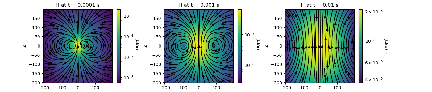
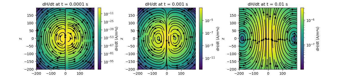
Magnetic Fields for a Transient Magnetic Dipole Source#
Here, we compute the magnetic field and its time-derivative for a transient magnetic dipole source in the z direction. Based on the geometry of the problem, we expect magnetic fields in the x and z directions, but none in the y direction.
# Defining electric dipole location and frequency
source_location = np.r_[0, 0, 0]
t = [1e-4, 1e-3, 1e-2]

# Defining observation locations (avoid placing observation at source)
x = np.arange(-201, 201, step=2.0)
y = np.r_[0]
z = x
observation_locations = utils.ndgrid(x, y, z)

# Define wholespace conductivity
sig = 1e0

# Plot the magnetic field
fig = plt.figure(figsize=(14, 3))
ax = 3 * [None]
cb = 3 * [None]
pc = 3 * [None]

for ii in range(0, 3):
    # Compute the fields
    Hx, Hy, Hz = TransientMagneticDipoleWholeSpace(
        observation_locations,
        source_location,
        sig,
        t[ii],
        moment="Z",
        fieldType="h",
        mu_r=1,
    )

    hxplt = Hx.reshape(x.size, z.size)
    hzplt = Hz.reshape(x.size, z.size)

    ax[ii] = fig.add_axes([0.1 + 0.28 * ii, 0.1, 0.2, 0.8])
    absH = np.sqrt(Hx**2 + Hy**2 + Hz**2)
    pc[ii] = ax[ii].pcolor(x, z, absH.reshape(x.size, z.size), norm=LogNorm())
    ax[ii].streamplot(x, z, hxplt.real, hzplt.real, color="k", density=1)
    ax[ii].set_xlim([x.min(), x.max()])
    ax[ii].set_ylim([z.min(), z.max()])
    ax[ii].set_title("H at t = {} s".format(t[ii]))
    ax[ii].set_xlabel("x")
    ax[ii].set_ylabel("z")
    cb[ii] = plt.colorbar(pc[ii], ax=ax[ii])
    cb[ii].set_label("H (A/m)")

# Plot the time-derivative
fig = plt.figure(figsize=(14, 3))
ax = 3 * [None]
cb = 3 * [None]
pc = 3 * [None]

for ii in range(0, 3):
    # Compute the fields
    dHdtx, dHdty, dHdtz = TransientMagneticDipoleWholeSpace(
        observation_locations,
        source_location,
        sig,
        t[ii],
        moment="Z",
        fieldType="dhdt",
        mu_r=1,
    )

    dhdtxplt = dHdtx.reshape(x.size, z.size)
    dhdtzplt = dHdtz.reshape(x.size, z.size)

    ax[ii] = fig.add_axes([0.1 + 0.28 * ii, 0.1, 0.2, 0.8])
    absdHdt = np.sqrt(dHdtx**2 + dHdty**2 + dHdtz**2)
    pc[ii] = ax[ii].pcolor(x, z, absdHdt.reshape(x.size, z.size), norm=LogNorm())
    ax[ii].streamplot(x, z, dhdtxplt.real, dhdtzplt.real, color="k", density=1)
    ax[ii].set_xlim([x.min(), x.max()])
    ax[ii].set_ylim([z.min(), z.max()])
    ax[ii].set_title("dH/dt at t = {} s".format(t[ii]))
    ax[ii].set_xlabel("x")
    ax[ii].set_ylabel("z")
    cb[ii] = plt.colorbar(pc[ii], ax=ax[ii])
    cb[ii].set_label("dH/dt (A/m*s)")
Electric Field from a Transient Electric Current Dipole Source#
Here, we compute the electric fields for a transient electric current dipole source in the z direction. Based on the geometry of the problem, we expect electric fields in the x and z directions, but none in the y direction.
# Defining electric dipole location and frequency
source_location = np.r_[0, 0, 0]
t = [1e-4, 1e-3, 1e-2]

# Defining observation locations (avoid placing observation at source)
x = np.arange(-201, 201, step=2.0)
y = np.r_[0]
z = x
observation_locations = utils.ndgrid(x, y, z)

# Define wholespace conductivity
sig = 1e0

fig = plt.figure(figsize=(14, 3))
ax = 3 * [None]
cb = 3 * [None]
pc = 3 * [None]

for ii in range(0, 3):
    # Compute the fields
    Ex, Ey, Ez = TransientElectricDipoleWholeSpace(
        observation_locations,
        source_location,
        sig,
        t[ii],
        moment="Z",
        fieldType="e",
        mu_r=1,
    )

    explt = Ex.reshape(x.size, z.size)
    ezplt = Ez.reshape(x.size, z.size)

    ax[ii] = fig.add_axes([0.1 + 0.28 * ii, 0.1, 0.2, 0.8])
    absE = np.sqrt(Ex**2 + Ey**2 + Ez**2)
    pc[ii] = ax[ii].pcolor(x, z, absE.reshape(x.size, z.size), norm=LogNorm())
    ax[ii].streamplot(x, z, explt.real, ezplt.real, color="k", density=1)
    ax[ii].set_xlim([x.min(), x.max()])
    ax[ii].set_ylim([z.min(), z.max()])
    ax[ii].set_title("E at t = {} s".format(t[ii]))
    ax[ii].set_xlabel("x")
    ax[ii].set_ylabel("z")
    cb[ii] = plt.colorbar(pc[ii], ax=ax[ii])
    cb[ii].set_label("E (V/m)")

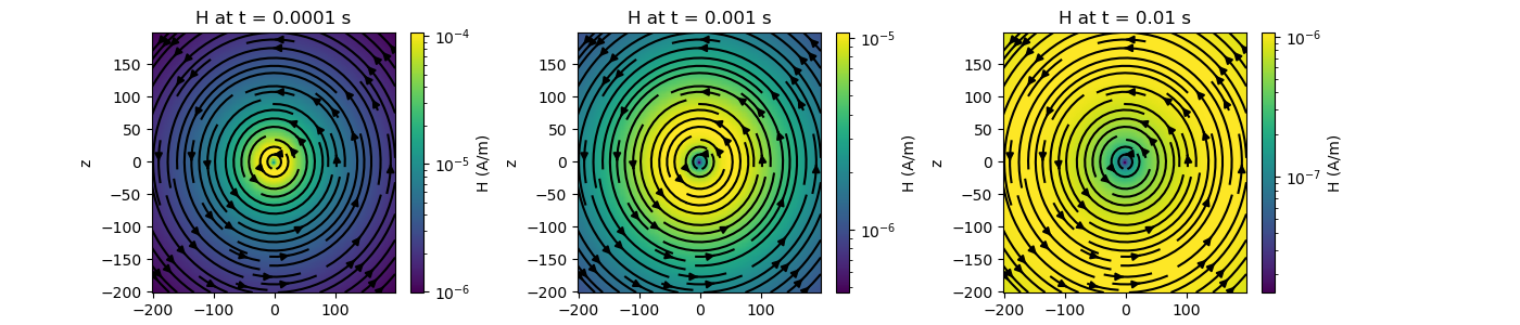
Magnetic Field from a Transient Electric Dipole Source#
Here, we compute the magnetic fields for a transient electric current dipole source in the y direction. Based on the geometry of the problem, we expect rotational magnetic fields in the x and z directions, but no fields in the y direction.
# Defining electric dipole location and frequency
source_location = np.r_[0, 0, 0]
t = [1e-4, 1e-3, 1e-2]

# Defining observation locations (avoid placing observation at source)
x = np.arange(-201, 201, step=2.0)
y = np.r_[0]
z = x
observation_locations = utils.ndgrid(x, y, z)

# Define wholespace conductivity
sig = 1e0

fig = plt.figure(figsize=(14, 3))
ax = 3 * [None]
cb = 3 * [None]
pc = 3 * [None]

for ii in range(0, 3):
    # Compute the fields
    Hx, Hy, Hz = TransientElectricDipoleWholeSpace(
        observation_locations,
        source_location,
        sig,
        t[ii],
        moment="Y",
        fieldType="h",
        mu_r=1,
    )

    hxplt = Hx.reshape(x.size, z.size)
    hzplt = Hz.reshape(x.size, z.size)

    ax[ii] = fig.add_axes([0.1 + 0.28 * ii, 0.1, 0.2, 0.8])
    absH = np.sqrt(Hx**2 + Hy**2 + Hz**2)
    pc[ii] = ax[ii].pcolor(x, z, absH.reshape(x.size, z.size), norm=LogNorm())
    ax[ii].streamplot(x, z, hxplt.real, hzplt.real, color="k", density=1)
    ax[ii].set_xlim([x.min(), x.max()])
    ax[ii].set_ylim([z.min(), z.max()])
    ax[ii].set_title("H at t = {} s".format(t[ii]))
    ax[ii].set_xlabel("x")
    ax[ii].set_ylabel("z")
    cb[ii] = plt.colorbar(pc[ii], ax=ax[ii])
    cb[ii].set_label("H (A/m)")
Total running time of the script: (0 minutes 8.007 seconds)
Estimated memory usage: 393 MB