1D Inversion of Time-Domain Data for a Single Sounding#

Here we use the module simpeg.electromangetics.time_domain_1d to invert time domain data and recover a 1D electrical conductivity model. In this tutorial, we focus on the following:

How to define sources and receivers from a survey file

How to define the survey

Sparse 1D inversion of with iteratively re-weighted least-squares

For this tutorial, we will invert 1D time domain data for a single sounding. The end product is layered Earth model which explains the data. The survey consisted of a horizontal loop with a radius of 6 m, located 20 m above the surface. The receiver measured the vertical component of the magnetic flux at the loop’s centre.

Import modules#

import os
import tarfile
import numpy as np
import matplotlib.pyplot as plt

from discretize import TensorMesh

import simpeg.electromagnetics.time_domain as tdem

from simpeg.utils import mkvc, plot_1d_layer_model
from simpeg import (
    maps,
    data,
    data_misfit,
    inverse_problem,
    regularization,
    optimization,
    directives,
    inversion,
    utils,
)

plt.rcParams.update({"font.size": 16, "lines.linewidth": 2, "lines.markersize": 8})

# sphinx_gallery_thumbnail_number = 2

Download Test Data File#

Here we provide the file path to the data we plan on inverting. The path to the data file is stored as a tar-file on our google cloud bucket: “https://storage.googleapis.com/simpeg/doc-assets/em1dtm.tar.gz”

# storage bucket where we have the data
data_source = "https://storage.googleapis.com/simpeg/doc-assets/em1dtm.tar.gz"

# download the data
downloaded_data = utils.download(data_source, overwrite=True)

# unzip the tarfile
tar = tarfile.open(downloaded_data, "r")
tar.extractall()
tar.close()

# path to the directory containing our data
dir_path = downloaded_data.split(".")[0] + os.path.sep

# files to work with
data_filename = dir_path + "em1dtm_data.txt"

Downloading https://storage.googleapis.com/simpeg/doc-assets/em1dtm.tar.gz
   saved to: /home/vsts/work/1/s/tutorials/08-tdem/em1dtm.tar.gz
Download completed!

Load Data and Plot#

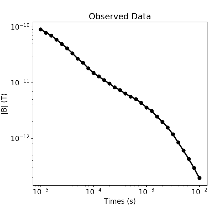
Here we load and plot the 1D sounding data. In this case, we have the B-field response to a step-off waveform.

# Load field data
dobs = np.loadtxt(str(data_filename), skiprows=1)

times = dobs[:, 0]
dobs = mkvc(dobs[:, -1])

fig = plt.figure(figsize=(7, 7))
ax = fig.add_axes([0.15, 0.15, 0.8, 0.75])
ax.loglog(times, np.abs(dobs), "k-o", lw=3)
ax.set_xlabel("Times (s)")
ax.set_ylabel("|B| (T)")
ax.set_title("Observed Data")

Text(0.5, 1.0, 'Observed Data')

Defining the Survey#

Here we demonstrate a general way to define the receivers, sources, waveforms and survey. For this tutorial, we define a single horizontal loop source as well a receiver which measures the vertical component of the magnetic flux.

# Source loop geometry
source_location = np.array([0.0, 0.0, 20.0])
source_orientation = "z"  # "x", "y" or "z"
source_current = 1.0  # peak current amplitude
source_radius = 6.0  # loop radius

# Receiver geometry
receiver_location = np.array([0.0, 0.0, 20.0])
receiver_orientation = "z"  # "x", "y" or "z"

# Receiver list
receiver_list = []
receiver_list.append(
    tdem.receivers.PointMagneticFluxDensity(
        receiver_location, times, orientation=receiver_orientation
    )
)

# Define the source waveform.
waveform = tdem.sources.StepOffWaveform()

# Sources
source_list = [
    tdem.sources.CircularLoop(
        receiver_list=receiver_list,
        location=source_location,
        waveform=waveform,
        current=source_current,
        radius=source_radius,
    )
]

# Survey
survey = tdem.Survey(source_list)

Assign Uncertainties and Define the Data Object#

Here is where we define the data that are inverted. The data are defined by the survey, the observation values and the uncertainties.

# 5% of the absolute value
uncertainties = 0.05 * np.abs(dobs) * np.ones(np.shape(dobs))

# Define the data object
data_object = data.Data(survey, dobs=dobs, standard_deviation=uncertainties)

Defining a 1D Layered Earth (1D Tensor Mesh)#

Here, we define the layer thicknesses for our 1D simulation. To do this, we use the TensorMesh class.

# Layer thicknesses
inv_thicknesses = np.logspace(0, 1.5, 25)

# Define a mesh for plotting and regularization.
mesh = TensorMesh([(np.r_[inv_thicknesses, inv_thicknesses[-1]])], "0")

Define a Starting and Reference Model#

Here, we create starting and/or reference models for the inversion as well as the mapping from the model space to the active cells. Starting and reference models can be a constant background value or contain a-priori structures. Here, the starting model is log(0.1) S/m.

Define log-conductivity values for each layer since our model is the log-conductivity. Don’t make the values 0! Otherwise the gradient for the 1st iteration is zero and the inversion will not converge.

# Define model. A resistivity (Ohm meters) or conductivity (S/m) for each layer.
starting_model = np.log(0.1 * np.ones(mesh.nC))

# Define mapping from model to active cells.
model_mapping = maps.ExpMap()

Define the Physics using a Simulation Object#

simulation = tdem.Simulation1DLayered(
    survey=survey, thicknesses=inv_thicknesses, sigmaMap=model_mapping
)

Define Inverse Problem#

The inverse problem is defined by 3 things:

Data Misfit: a measure of how well our recovered model explains the field data

Regularization: constraints placed on the recovered model and a priori information

Optimization: the numerical approach used to solve the inverse problem

# Define the data misfit. Here the data misfit is the L2 norm of the weighted
# residual between the observed data and the data predicted for a given model.
# The weighting is defined by the reciprocal of the uncertainties.
dmis = data_misfit.L2DataMisfit(simulation=simulation, data=data_object)
dmis.W = 1.0 / uncertainties

# Define the regularization (model objective function)
reg_map = maps.IdentityMap(nP=mesh.nC)
reg = regularization.Sparse(mesh, mapping=reg_map, alpha_s=0.01, alpha_x=1.0)

# set reference model
reg.reference_model = starting_model

# Define sparse and blocky norms p, q
reg.norms = [1, 0]

# Define how the optimization problem is solved. Here we will use an inexact
# Gauss-Newton approach that employs the conjugate gradient solver.
opt = optimization.ProjectedGNCG(maxIter=100, maxIterLS=20, cg_maxiter=30, cg_rtol=1e-3)

# Define the inverse problem
inv_prob = inverse_problem.BaseInvProblem(dmis, reg, opt)

Define Inversion Directives#

Here we define any directiveas that are carried out during the inversion. This includes the cooling schedule for the trade-off parameter (beta), stopping criteria for the inversion and saving inversion results at each iteration.

# Defining a starting value for the trade-off parameter (beta) between the data
# misfit and the regularization.
starting_beta = directives.BetaEstimate_ByEig(beta0_ratio=1e2)

# Update the preconditionner
update_Jacobi = directives.UpdatePreconditioner()

# Options for outputting recovered models and predicted data for each beta.
save_iteration = directives.SaveOutputEveryIteration(save_txt=False)

# Directives for the IRLS
update_IRLS = directives.UpdateIRLS(max_irls_iterations=30, irls_cooling_factor=1.5)

# Updating the preconditionner if it is model dependent.
update_jacobi = directives.UpdatePreconditioner()

# Add sensitivity weights
sensitivity_weights = directives.UpdateSensitivityWeights()

# The directives are defined as a list.
directives_list = [
    sensitivity_weights,
    starting_beta,
    save_iteration,
    update_IRLS,
    update_jacobi,
]

/home/vsts/work/1/s/simpeg/directives/_directives.py:1865: FutureWarning:

SaveEveryIteration.save_txt has been deprecated, please use SaveEveryIteration.on_disk. It will be removed in version 0.26.0 of SimPEG.

/home/vsts/work/1/s/simpeg/directives/_directives.py:1866: FutureWarning:

SaveEveryIteration.save_txt has been deprecated, please use SaveEveryIteration.on_disk. It will be removed in version 0.26.0 of SimPEG.

Running the Inversion#

To define the inversion object, we need to define the inversion problem and the set of directives. We can then run the inversion.

# Here we combine the inverse problem and the set of directives
inv = inversion.BaseInversion(inv_prob, directives_list)

# Run the inversion
recovered_model = inv.run(starting_model)

Running inversion with SimPEG v0.25.0
================================================= Projected GNCG =================================================
  #     beta     phi_d     phi_m       f      |proj(x-g)-x|  LS   iter_CG   CG |Ax-b|/|b|  CG |Ax-b|   Comment
-----------------------------------------------------------------------------------------------------------------
1.68e+04  4.01e+03  0.00e+00  4.01e+03                         0           inf          inf
1.68e+04  1.51e+03  4.16e-02  2.21e+03    8.04e+02      0      18       3.01e-04     2.42e-01
8.40e+03  3.35e+02  1.03e-01  1.20e+03    6.06e+02      0      15       5.08e-04     3.07e-01
4.20e+03  1.45e+02  1.10e-01  6.08e+02    4.58e+02      0      16       4.20e-04     1.92e-01
2.10e+03  5.29e+01  1.15e-01  2.95e+02    4.95e+02      0      10       6.44e-04     3.19e-01
1.05e+03  1.57e+01  1.18e-01  1.40e+02    3.55e+02      0      14       8.49e-04     3.01e-01
Reached starting chifact with l2-norm regularization: Start IRLS steps...
irls_threshold 2.7411069809877096
1.05e+03  2.35e+01  1.06e-01  1.35e+02    1.98e+02      0      15       5.80e-04     1.15e-01
1.74e+03  1.57e+01  1.02e-01  1.94e+02    4.05e+02      0      12       3.17e-04     1.29e-01
3.46e+03  2.38e+01  1.06e-01  3.91e+02    3.09e+02      0      12       6.66e-04     2.06e-01
5.72e+03  4.39e+01  1.22e-01  7.39e+02    2.67e+02      0      11       5.74e-04     1.53e-01
4.16e+03  4.37e+01  1.41e-01  6.30e+02    4.25e+01      0      13       8.33e-04     3.54e-02
3.04e+03  4.16e+01  1.56e-01  5.15e+02    5.62e+01      0      13       9.16e-04     5.15e-02
2.27e+03  3.84e+01  1.62e-01  4.07e+02    5.64e+01      0      14       7.47e-04     4.21e-02
1.77e+03  3.43e+01  1.59e-01  3.16e+02    5.08e+01      0      15       7.80e-04     3.96e-02
1.46e+03  3.26e+01  1.47e-01  2.48e+02    4.68e+01      0      16       3.62e-04     1.70e-02
1.46e+03  3.52e+01  1.31e-01  2.26e+02    1.45e+02      0      15       6.03e-04     8.73e-02
1.19e+03  3.85e+01  1.14e-01  1.74e+02    2.22e+02      0      14       3.71e-04     8.22e-02
9.27e+02  3.69e+01  1.00e-01  1.30e+02    2.97e+02      0      10       5.89e-04     1.75e-01
7.37e+02  3.69e+01  9.08e-02  1.04e+02    1.47e+02      0      11       3.38e-04     4.97e-02
5.86e+02  3.73e+01  8.31e-02  8.60e+01    2.99e+01      0      11       8.76e-04     2.62e-02
4.63e+02  3.73e+01  7.72e-02  7.31e+01    1.47e+01      0      11       4.41e-04     6.47e-03
3.66e+02  3.70e+01  7.37e-02  6.40e+01    1.60e+01      0      12       3.68e-04     5.89e-03
2.91e+02  3.62e+01  7.27e-02  5.73e+01    2.43e+01      0      13       6.69e-04     1.62e-02
2.34e+02  3.47e+01  7.47e-02  5.22e+01    3.39e+01      0      14       4.63e-04     1.57e-02
1.92e+02  3.25e+01  7.95e-02  4.77e+01    3.88e+01      0      15       9.05e-04     3.51e-02
1.92e+02  3.07e+01  8.08e-02  4.62e+01    2.86e+01      0      16       1.07e-04     3.08e-03
1.92e+02  2.95e+01  8.11e-02  4.51e+01    1.96e+01      0      16       7.89e-05     1.55e-03
Minimum decrease in regularization. End of IRLS
------------------------- STOP! -------------------------
: |fc-fOld| = 1.5723e-01 <= tolF*(1+|f0|) = 4.0084e+02
: |xc-x_last| = 1.7413e-02 <= tolX*(1+|x0|) = 1.2741e+00
: |proj(x-g)-x|    = 1.9596e+01 <= tolG          = 1.0000e-01
: |proj(x-g)-x|    = 1.9596e+01 <= 1e3*eps       = 1.0000e-02
: maxIter   =     100    <= iter          =     26
------------------------- DONE! -------------------------

Plotting Results#

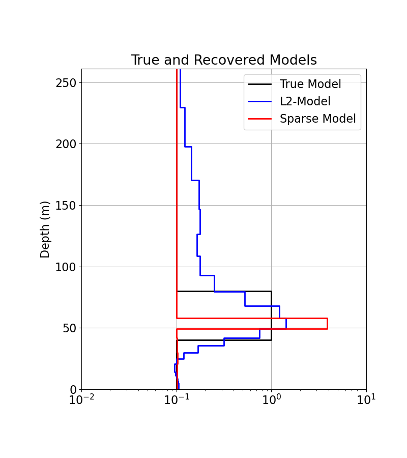
# Load the true model and layer thicknesses
true_model = np.array([0.1, 1.0, 0.1])
true_layers = np.r_[40.0, 40.0, 160.0]

# Extract Least-Squares model
l2_model = inv_prob.l2model
print(np.shape(l2_model))

# Plot true model and recovered model
fig = plt.figure(figsize=(8, 9))
x_min = np.min(
    np.r_[model_mapping * recovered_model, model_mapping * l2_model, true_model]
)
x_max = np.max(
    np.r_[model_mapping * recovered_model, model_mapping * l2_model, true_model]
)

ax1 = fig.add_axes([0.2, 0.15, 0.7, 0.7])
plot_1d_layer_model(true_layers, true_model, ax=ax1, show_layers=False, color="k")
plot_1d_layer_model(
    mesh.h[0], model_mapping * l2_model, ax=ax1, show_layers=False, color="b"
)
plot_1d_layer_model(
    mesh.h[0], model_mapping * recovered_model, ax=ax1, show_layers=False, color="r"
)
ax1.set_xlim(0.01, 10)
ax1.grid()
ax1.set_title("True and Recovered Models")
ax1.legend(["True Model", "L2-Model", "Sparse Model"])
plt.gca().invert_yaxis()

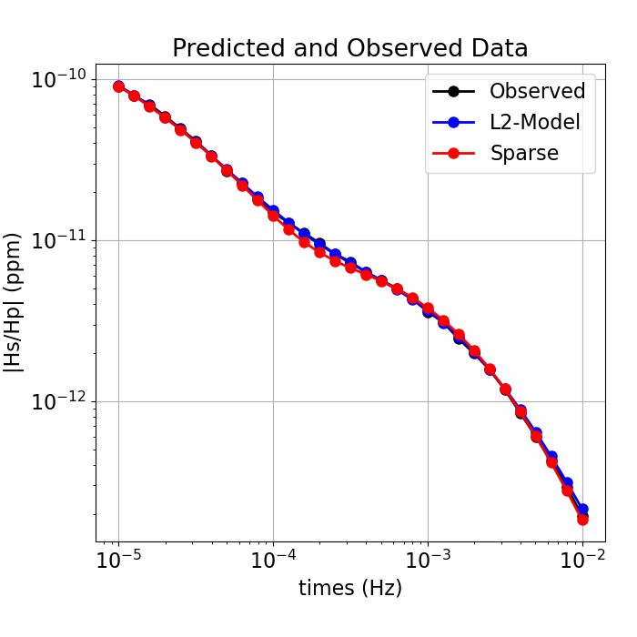
# Plot predicted and observed data
dpred_l2 = simulation.dpred(l2_model)
dpred_final = simulation.dpred(recovered_model)

fig = plt.figure(figsize=(7, 7))
ax1 = fig.add_axes([0.15, 0.15, 0.8, 0.75])
ax1.loglog(times, np.abs(dobs), "k-o")
ax1.loglog(times, np.abs(dpred_l2), "b-o")
ax1.loglog(times, np.abs(dpred_final), "r-o")
ax1.grid()
ax1.set_xlabel("times (Hz)")
ax1.set_ylabel("|Hs/Hp| (ppm)")
ax1.set_title("Predicted and Observed Data")
ax1.legend(["Observed", "L2-Model", "Sparse"], loc="upper right")
plt.show()