Note
Go to the end to download the full example code.
Sparse Inversion with Iteratively Re-Weighted Least-Squares#
Least-squares inversion produces smooth models which may not be an accurate representation of the true model. Here we demonstrate the basics of inverting for sparse and/or blocky models. Here, we used the iteratively reweighted least-squares approach. For this tutorial, we focus on the following:
Defining the forward problem
Defining the inverse problem (data misfit, regularization, optimization)
Defining the paramters for the IRLS algorithm
Specifying directives for the inversion
Recovering a set of model parameters which explains the observations
import numpy as np
import matplotlib.pyplot as plt

from discretize import TensorMesh

from simpeg import (
    simulation,
    maps,
    data_misfit,
    directives,
    optimization,
    regularization,
    inverse_problem,
    inversion,
)

# sphinx_gallery_thumbnail_number = 3
Defining the Model and Mapping#
Here we generate a synthetic model and a mappig which goes from the model space to the row space of our linear operator.
nParam = 100  # Number of model paramters

# A 1D mesh is used to define the row-space of the linear operator.
mesh = TensorMesh([nParam])

# Creating the true model
true_model = np.zeros(mesh.nC)
true_model[mesh.cell_centers_x > 0.3] = 1.0
true_model[mesh.cell_centers_x > 0.45] = -0.5
true_model[mesh.cell_centers_x > 0.6] = 0

# Mapping from the model space to the row space of the linear operator
model_map = maps.IdentityMap(mesh)

# Plotting the true model
fig = plt.figure(figsize=(8, 5))
ax = fig.add_subplot(111)
ax.plot(mesh.cell_centers_x, true_model, "b-")
ax.set_ylim([-2, 2])
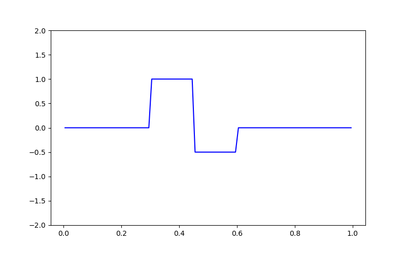
(-2.0, 2.0)
Defining the Linear Operator#
Here we define the linear operator with dimensions (nData, nParam). In practive, you may have a problem-specific linear operator which you would like to construct or load here.
# Number of data observations (rows)
nData = 20

# Create the linear operator for the tutorial. The columns of the linear operator
# represents a set of decaying and oscillating functions.
jk = np.linspace(1.0, 60.0, nData)
p = -0.25
q = 0.25


def g(k):
    return np.exp(p * jk[k] * mesh.cell_centers_x) * np.cos(
        np.pi * q * jk[k] * mesh.cell_centers_x
    )


G = np.empty((nData, nParam))

for i in range(nData):
    G[i, :] = g(i)

# Plot the columns of G
fig = plt.figure(figsize=(8, 5))
ax = fig.add_subplot(111)
for i in range(G.shape[0]):
    ax.plot(G[i, :])

ax.set_title("Columns of matrix G")
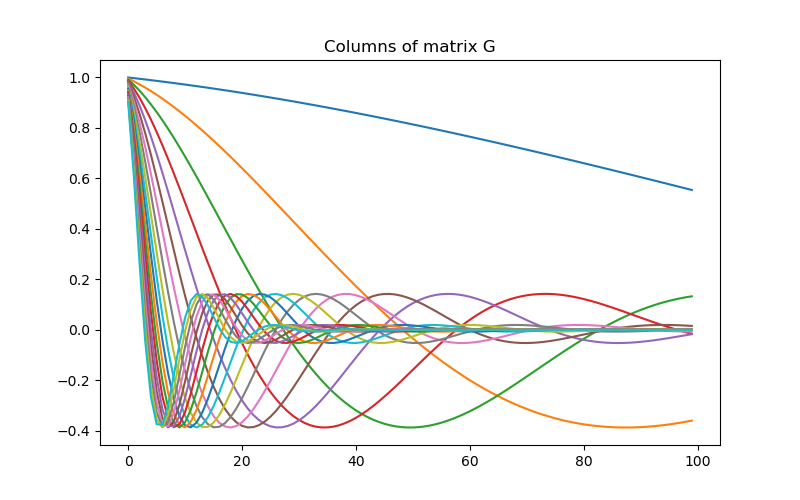
Text(0.5, 1.0, 'Columns of matrix G')
Defining the Simulation#
The simulation defines the relationship between the model parameters and predicted data.
Predict Synthetic Data#
Here, we use the true model to create synthetic data which we will subsequently invert.
# Standard deviation of Gaussian noise being added
std = 0.02
np.random.seed(1)

# Create a SimPEG data object
data_obj = sim.make_synthetic_data(true_model, noise_floor=std, add_noise=True)
Define the Inverse Problem#
The inverse problem is defined by 3 things:
Data Misfit: a measure of how well our recovered model explains the field data
Regularization: constraints placed on the recovered model and a priori information
Optimization: the numerical approach used to solve the inverse problem
# Define the data misfit. Here the data misfit is the L2 norm of the weighted
# residual between the observed data and the data predicted for a given model.
# Within the data misfit, the residual between predicted and observed data are
# normalized by the data's standard deviation.
dmis = data_misfit.L2DataMisfit(simulation=sim, data=data_obj)

# Define the regularization (model objective function). Here, 'p' defines the
# the norm of the smallness term and 'q' defines the norm of the smoothness
# term.
reg = regularization.Sparse(mesh, mapping=model_map)
reg.reference_model = np.zeros(nParam)
p = 0.0
q = 0.0
reg.norms = [p, q]

# Define how the optimization problem is solved.
opt = optimization.ProjectedGNCG(
    maxIter=100, lower=-2.0, upper=2.0, maxIterLS=20, cg_maxiter=30, cg_rtol=1e-3
)

# Here we define the inverse problem that is to be solved
inv_prob = inverse_problem.BaseInvProblem(dmis, reg, opt)
Define Inversion Directives#
Here we define any directiveas that are carried out during the inversion. This includes the cooling schedule for the trade-off parameter (beta), stopping criteria for the inversion and saving inversion results at each iteration.
# Add sensitivity weights but don't update at each beta
sensitivity_weights = directives.UpdateSensitivityWeights(every_iteration=False)

# Reach target misfit for L2 solution, then use IRLS until model stops changing.
IRLS = directives.UpdateIRLS(max_irls_iterations=40, f_min_change=1e-4)

# Defining a starting value for the trade-off parameter (beta) between the data
# misfit and the regularization.
starting_beta = directives.BetaEstimate_ByEig(beta0_ratio=1e0)

# Update the preconditionner
update_Jacobi = directives.UpdatePreconditioner()

# Save output at each iteration
saveDict = directives.SaveOutputEveryIteration(save_txt=False)

# Define the directives as a list
directives_list = [
    sensitivity_weights,
    IRLS,
    starting_beta,
    update_Jacobi,
    saveDict,
]
/home/vsts/work/1/s/simpeg/directives/_directives.py:1865: FutureWarning: SaveEveryIteration.save_txt has been deprecated, please use SaveEveryIteration.on_disk. It will be removed in version 0.26.0 of SimPEG.
  self.save_txt = save_txt
/home/vsts/work/1/s/simpeg/directives/_directives.py:1866: FutureWarning: SaveEveryIteration.save_txt has been deprecated, please use SaveEveryIteration.on_disk. It will be removed in version 0.26.0 of SimPEG.
  on_disk = self.save_txt
Setting a Starting Model and Running the Inversion#
To define the inversion object, we need to define the inversion problem and the set of directives. We can then run the inversion.
# Here we combine the inverse problem and the set of directives
inv = inversion.BaseInversion(inv_prob, directives_list)

# Starting model
starting_model = 1e-4 * np.ones(nParam)

# Run inversion
recovered_model = inv.run(starting_model)
Running inversion with SimPEG v0.25.2
================================================= Projected GNCG =================================================
  #     beta     phi_d     phi_m       f      |proj(x-g)-x|  LS   iter_CG   CG |Ax-b|/|b|  CG |Ax-b|   Comment
-----------------------------------------------------------------------------------------------------------------
   0  1.70e+06  3.70e+03  1.02e-09  3.70e+03                         0           inf          inf
   1  1.70e+06  1.89e+03  3.80e-04  2.53e+03    1.96e+01      0      8        3.89e-04     1.78e+00
   2  8.48e+05  1.30e+03  8.83e-04  2.05e+03    1.90e+01      0      9        2.58e-04     2.06e-01
   3  4.24e+05  7.64e+02  1.78e-03  1.52e+03    1.86e+01      0      10       5.04e-04     2.98e-01
   4  2.12e+05  3.81e+02  3.05e-03  1.03e+03    1.76e+01      0      11       7.81e-04     3.25e-01
   5  1.06e+05  1.62e+02  4.48e-03  6.37e+02    1.51e+01      0      14       4.58e-04     1.24e-01
   6  5.30e+04  6.17e+01  5.79e-03  3.68e+02    1.39e+01      0      16       8.88e-04     1.44e-01
   7  2.65e+04  2.29e+01  6.78e-03  2.03e+02    1.30e+01      0      20       8.81e-04     8.08e-02
   8  1.32e+04  9.70e+00  7.46e-03  1.08e+02    1.07e+01      0      29       7.21e-04     3.58e-02
Reached starting chifact with l2-norm regularization: Start IRLS steps...
irls_threshold 1.2492122951221412
   9  1.32e+04  1.70e+01  9.22e-03  1.39e+02    1.51e+01      0      28       9.49e-04     2.98e-02
  10  2.10e+04  3.90e+01  9.17e-03  2.32e+02    1.83e+01      0      20       8.85e-04     6.24e-02
  11  1.33e+04  3.12e+01  1.07e-02  1.74e+02    9.92e+00      0      21       9.60e-04     2.92e-02
  12  9.23e+03  2.71e+01  1.19e-02  1.37e+02    7.94e+00      0      23       9.19e-04     1.69e-02
  13  6.87e+03  2.40e+01  1.28e-02  1.12e+02    6.97e+00      0      24       7.49e-04     1.00e-02
  14  5.44e+03  2.13e+01  1.32e-02  9.29e+01    6.33e+00      0      24       7.07e-04     7.65e-03
  15  5.44e+03  2.18e+01  1.24e-02  8.94e+01    7.46e+00      0      24       5.63e-04     4.55e-03
  16  5.44e+03  2.20e+01  1.16e-02  8.51e+01    7.87e+00      0      23       8.38e-04     7.24e-03
  17  5.44e+03  2.17e+01  1.06e-02  7.95e+01    8.03e+00      0      22       3.97e-04     3.59e-03
  18  5.44e+03  2.10e+01  9.59e-03  7.31e+01    8.25e+00      0      21       9.08e-04     8.50e-03
  19  5.44e+03  1.99e+01  8.52e-03  6.63e+01    8.62e+00      0      18       5.45e-04     5.42e-03
  20  5.44e+03  1.83e+01  7.36e-03  5.83e+01    8.73e+00      0      19       9.93e-04     1.06e-02
  21  5.44e+03  1.67e+01  6.40e-03  5.15e+01    9.45e+00      0      21       6.34e-04     7.32e-03
  22  8.70e+03  1.94e+01  4.87e-03  6.18e+01    1.62e+01      0      18       9.86e-04     3.68e-02
  23  8.70e+03  1.90e+01  4.23e-03  5.58e+01    9.50e+00      0      20       8.72e-04     1.25e-02
  24  8.70e+03  1.85e+01  3.81e-03  5.17e+01    1.10e+01      0      20       4.24e-04     7.72e-03
  25  8.70e+03  1.80e+01  3.44e-03  4.79e+01    1.17e+01      0      20       7.23e-04     1.58e-02
  26  8.70e+03  1.76e+01  3.01e-03  4.38e+01    1.70e+01      0      18       4.42e-04     1.84e-02
  27  1.36e+04  1.88e+01  2.37e-03  5.11e+01    1.67e+01      0      16       4.77e-04     3.01e-02
  28  1.36e+04  1.82e+01  2.01e-03  4.56e+01    1.23e+01      0      16       9.36e-04     3.13e-02
  29  1.36e+04  1.73e+01  1.68e-03  4.02e+01    1.19e+01      0      18       7.57e-04     2.36e-02
  30  2.15e+04  1.77e+01  1.32e-03  4.60e+01    1.72e+01      0      17       6.51e-04     6.39e-02
  31  3.37e+04  1.84e+01  1.06e-03  5.42e+01    1.78e+01      0      15       9.18e-04     1.33e-01
  32  3.37e+04  1.80e+01  9.01e-04  4.84e+01    1.36e+01      0      22       3.39e-04     1.65e-02
  33  3.37e+04  1.75e+01  7.53e-04  4.29e+01    1.61e+01      0      20       5.42e-04     3.27e-02
  34  5.29e+04  1.81e+01  6.04e-04  5.01e+01    1.76e+01      0      19       7.16e-04     1.80e-01
  35  5.29e+04  1.79e+01  5.09e-04  4.48e+01    1.38e+01      0      23       6.38e-04     4.70e-02
  36  8.26e+04  1.85e+01  4.08e-04  5.21e+01    1.84e+01      0      19       7.73e-04     2.64e-01
  37  8.26e+04  1.83e+01  3.40e-04  4.64e+01    1.39e+01      0      21       2.56e-04     2.41e-02
  38  8.26e+04  1.79e+01  2.80e-04  4.10e+01    1.38e+01      0      19       7.43e-04     8.92e-02
  39  1.29e+05  1.81e+01  2.23e-04  4.68e+01    1.83e+01      0      21       4.32e-04     2.43e-01
  40  1.29e+05  1.79e+01  1.88e-04  4.21e+01    1.37e+01      0      24       2.92e-04     5.95e-02
  41  2.01e+05  1.79e+01  1.53e-04  4.86e+01    1.94e+01      0      19       8.97e-04     4.05e-01
  42  3.13e+05  1.83e+01  1.27e-04  5.80e+01    1.81e+01      0      21       3.72e-04     1.67e-01
  43  3.13e+05  1.82e+01  1.07e-04  5.17e+01    1.36e+01      0      24       3.23e-04     3.35e-02
  44  3.13e+05  1.78e+01  8.93e-05  4.58e+01    1.33e+01      0      25       3.14e-04     3.12e-02
  45  4.88e+05  1.80e+01  7.35e-05  5.39e+01    1.88e+01      0      22       3.15e-04     1.52e-01
  46  4.88e+05  1.78e+01  6.21e-05  4.81e+01    1.35e+01      0      23       2.39e-04     2.54e-02
  47  7.63e+05  1.81e+01  5.09e-05  5.69e+01    1.79e+01      0      22       3.91e-04     1.84e-01
  48  7.63e+05  1.79e+01  4.29e-05  5.07e+01    1.37e+01      0      25       6.42e-04     6.90e-02
Reach maximum number of IRLS cycles: 40
------------------------- STOP! -------------------------
1 : |fc-fOld| = 1.4670e-01 <= tolF*(1+|f0|) = 3.6979e+02
0 : |xc-x_last| = 1.1429e-01 <= tolX*(1+|x0|) = 1.0010e-01
0 : |proj(x-g)-x|    = 1.3666e+01 <= tolG          = 1.0000e-01
0 : |proj(x-g)-x|    = 1.3666e+01 <= 1e3*eps       = 1.0000e-02
0 : maxIter   =     100    <= iter          =     48
------------------------- DONE! -------------------------
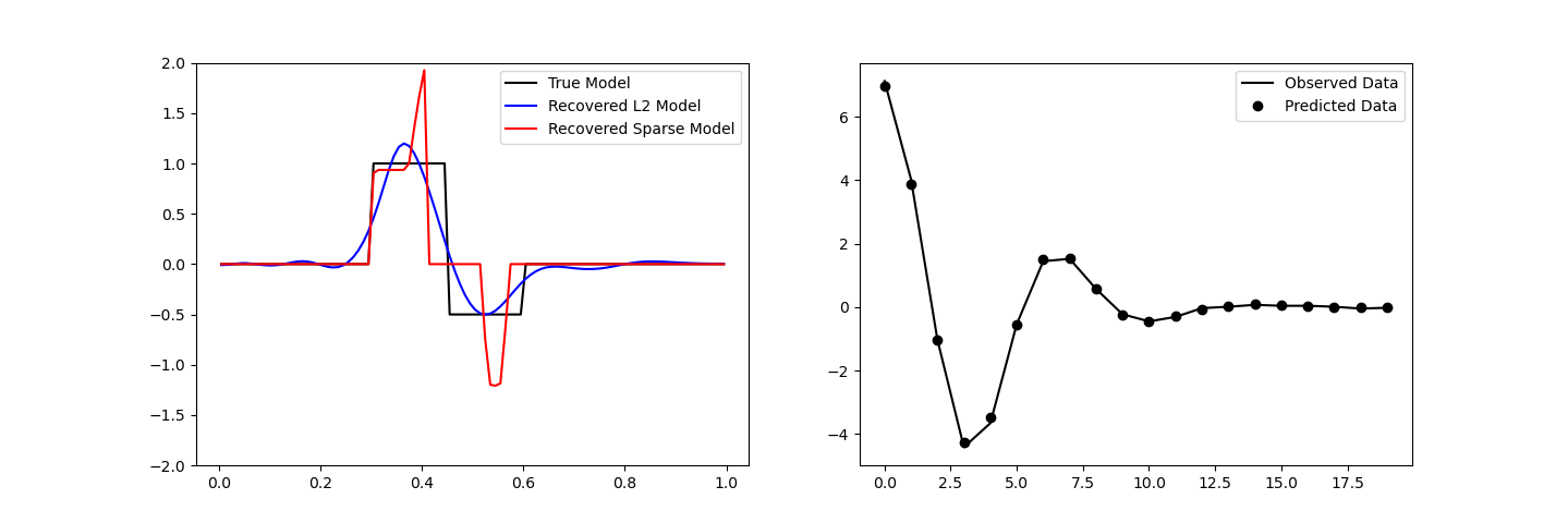
Plotting Results#
fig, ax = plt.subplots(1, 2, figsize=(12 * 1.2, 4 * 1.2))

# True versus recovered model
ax[0].plot(mesh.cell_centers_x, true_model, "k-")
ax[0].plot(mesh.cell_centers_x, inv_prob.l2model, "b-")
ax[0].plot(mesh.cell_centers_x, recovered_model, "r-")
ax[0].legend(("True Model", "Recovered L2 Model", "Recovered Sparse Model"))
ax[0].set_ylim([-2, 2])

# Observed versus predicted data
ax[1].plot(data_obj.dobs, "k-")
ax[1].plot(inv_prob.dpred, "ko")
ax[1].legend(("Observed Data", "Predicted Data"))

# Plot convergence
fig = plt.figure(figsize=(9, 5))
ax = fig.add_axes([0.2, 0.1, 0.7, 0.85])
ax.plot(saveDict.phi_d, "k", lw=2)

twin = ax.twinx()
twin.plot(saveDict.phi_m, "k--", lw=2)
ax.plot(
    np.r_[IRLS.metrics.start_irls_iter, IRLS.metrics.start_irls_iter],
    np.r_[0, np.max(saveDict.phi_d)],
    "k:",
)
ax.text(
    IRLS.metrics.start_irls_iter,
    0.0,
    "IRLS Start",
    va="bottom",
    ha="center",
    rotation="vertical",
    size=12,
    bbox={"facecolor": "white"},
)

ax.set_ylabel(r"$\phi_d$", size=16, rotation=0)
ax.set_xlabel("Iterations", size=14)
twin.set_ylabel(r"$\phi_m$", size=16, rotation=0)
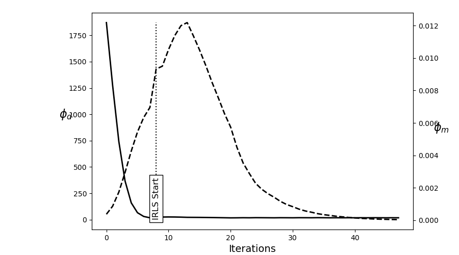
Text(865.1527777777777, 0.5, '$\\phi_m$')
Total running time of the script: (0 minutes 28.405 seconds)
Estimated memory usage: 325 MB