SimPEG.meta.MetaSimulation

class SimPEG.meta.MetaSimulation(simulations, mappings)

Bases: BaseSimulation

Combine multiple simulations into a single one.

This class is used to encapsulate multiple simulations into a single simulation. Each simulation and mapping pair will perform its own work, then concatenate the results together.

For each mapping and simulation pair, given a model, this first applies the mapping, then passes the resulting model to the simulation.

With the proper mappings this can be useful for setting up time-lapse, tiled, stitched, or any other simulation that can be broken into many individual simulations.

Parameters:

simulations(n_sim) list of SimPEG.simulation.BaseSimulation

The list of unique simulations that each handle a piece of the problem.

mappings(n_sim) list of SimPEG.maps.IdentityMap

The map for every simulation. Every map should accept the same length model, and output a model appropriate for its paired simulation.

Examples

Create a list of 1D simulations that perform a piece of a stitched problem.

>>> from SimPEG.simulation import ExponentialSinusoidSimulation
>>> from SimPEG import maps
>>> from SimPEG.meta import MetaSimulation
>>> from discretize import TensorMesh
>>> import matplotlib.pyplot as plt

Create a mesh for space and time, then one that represents the full dimensionality of the model. >>> mesh_space = TensorMesh([100]) >>> mesh_time = TensorMesh([5]) >>> full_mesh = TensorMesh([5, 100])

Lets say we have observations at 5 locations in time. For simplicity we will just use the same times from the time mesh, but this is not required. Then create a simulation for each of these times. We also create an operator that maps the model in full space to the model for each simulation. >>> obs_times = mesh_time.cell_centers_x >>> sims, mappings = [], [] >>> for time in obs_times: … sims.append(ExponentialSinusoidSimulation( … mesh=mesh_space, … model_map=maps.IdentityMap(), … )) … ccs = mesh_space.cell_centers … p_ave = full_mesh.get_interpolation_matrix( … np.c_[np.full_like(ccs, time), ccs] … ) … mappings.append(maps.LinearMap(p_ave)) >>> sim = MetaSimulation(sims, mappings)

This simulation acts like a single simulation, which can be used for modeling and inversion. This model is a moving box car. >>> true_model = np.zeros(full_mesh.shape_cells) >>> speed, start, width = 0.8, 0.1, 0.2 >>> for i, time in enumerate(mesh_time.cell_centers): … center = speed * time + start … in_box = np.abs(mesh_space.cell_centers - center) <= width/2 … true_model[i, in_box] = 1.0 >>> true_model = true_model.reshape(-1, order=’F’)

Then use the simulation to create data. >>> d_pred = sim.dpred(true_model) >>> plt.plot(d_pred.reshape(5, -1).T) >>> plt.show()

(Source code, png, pdf)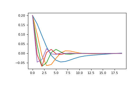

Attributes

clean_on_model_update	A list of solver objects to clean when the model is updated
counter	SimPEG Counter object to store iterations and run-times.
deleteTheseOnModelUpdate	A list of properties stored on this object to delete when the model is updated
mappings	The mappings paired to each simulation.
mesh	Mesh for the simulation.
model	The inversion model.
needs_model	True if a model is necessary
sensitivity_path	Path to directory where sensitivity file is stored.
simulations	The list of simulations.
solver	Numerical solver used in the forward simulation.
solver_opts	Solver-specific parameters.
survey	The survey for the simulation.
verbose	Verbose progress printout.

Methods

Jtvec(m, v[, f])	Compute the Jacobian transpose times a vector for the model provided.
Jtvec_approx(m, v[, f])	Approximation of the Jacobian transpose times a vector for the model provided.
Jvec(m, v[, f])	Compute the Jacobian times a vector for the model provided.
Jvec_approx(m, v[, f])	Approximation of the Jacobian times a vector for the model provided.
dpred([m, f])	Predicted data for the model provided.
fields(m)	Create fields for every simulation.
getJtJdiag(m[, W, f])	Return the squared sum of columns of the Jacobian.
make_synthetic_data(m[, relative_error, ...])	Make synthetic data for the model and Gaussian noise provided.
residual(m, dobs[, f])	The data residual.