Note
Go to the end to download the full example code
Maps: ComboMaps#
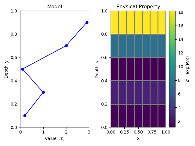
We will use an example where we want a 1D layered earth as our model,
but we want to map this to a 2D discretization to do our forward
modeling. We will also assume that we are working in log conductivity
still, so after the transformation we map to conductivity space.
To do this we will introduce the vertical 1D map
(SimPEG.maps.SurjectVertical1D), which does the first part of
what we just described. The second part will be done by the
SimPEG.maps.ExpMap described above.
1M = discretize.TensorMesh([7,5])
2v1dMap = maps.SurjectVertical1D(M)
3expMap = maps.ExpMap(M)
4myMap = expMap * v1dMap
5m = np.r_[0.2,1,0.1,2,2.9] # only 5 model parameters!
6sig = myMap * m
If you noticed, it was pretty easy to combine maps. What is even cooler is that the derivatives also are made for you (if everything goes right). Just to be sure that the derivative is correct, you should always run the test on the mapping that you create.

import discretize
from SimPEG import maps
import numpy as np
import matplotlib.pyplot as plt


def run(plotIt=True):
    M = discretize.TensorMesh([7, 5])
    v1dMap = maps.SurjectVertical1D(M)
    expMap = maps.ExpMap(M)
    myMap = expMap * v1dMap
    m = np.r_[0.2, 1, 0.1, 2, 2.9]  # only 5 model parameters!
    sig = myMap * m

    if not plotIt:
        return

    figs, axs = plt.subplots(1, 2)
    axs[0].plot(m, M.cell_centers_y, "b-o")
    axs[0].set_title("Model")
    axs[0].set_ylabel("Depth, y")
    axs[0].set_xlabel("Value, $m_i$")
    axs[0].set_xlim(0, 3)
    axs[0].set_ylim(0, 1)
    clbar = plt.colorbar(
        M.plot_image(sig, ax=axs[1], grid=True, grid_opts=dict(color="grey"))[0]
    )
    axs[1].set_title("Physical Property")
    axs[1].set_ylabel("Depth, y")
    clbar.set_label(r"$\sigma = \exp(\mathbf{P}m)$")
    plt.tight_layout()


if __name__ == "__main__":
    run()
    plt.show()
Total running time of the script: (0 minutes 0.355 seconds)
Estimated memory usage: 9 MB