SimPEG.maps.ParametricPolyMap#
- class SimPEG.maps.ParametricPolyMap(mesh, order, logSigma=True, normal='X', actInd=None, slope=10000.0)[source]#
Bases:
IdentityMapMapping for 2 layer model whose interface is defined by a polynomial.
This mapping is used when the cells lying below the Earth’s surface can be parameterized by a 2 layer model whose interface is defined by a polynomial function. The model is defined by the physical property values for each unit (\(\sigma_1\) and \(\sigma_2\)) and the coefficients for the polynomial function (\(\mathbf{c}\)).
For a 2D mesh , the interface is defined by a polynomial function of the form:
\[p(x) = \sum_{i=0}^N c_i x^i\]where \(c_i\) are the polynomial coefficients and \(N\) is the order of the polynomial. In this case, the model is defined as
\[\mathbf{m} = [\sigma_1, \;\sigma_2,\; c_0 ,\;\ldots\; ,\; c_N]\]The mapping \(\mathbf{u}(\mathbf{m})\) from the model to the mesh is given by:
\[\mathbf{u}(\mathbf{m}) = \sigma_1 + (\sigma_2 - \sigma_1) \bigg [ \frac{1}{2} + \pi^{-1} \arctan \bigg ( a \Big ( \mathbf{p}(\mathbf{x_c}) - \mathbf{y_c} \Big ) \bigg ) \bigg ]\]where \(\mathbf{x_c}\) and \(\mathbf{y_c}\) are vectors containing the x and y cell center locations for all active cells in the mesh, and \(a\) is a parameter which defines the sharpness of the boundary between the two layers. \(\mathbf{p}(\mathbf{x_c})\) evaluates the polynomial function for every element in \(\mathbf{x_c}\).
For a 3D mesh , the interface is defined by a 2D polynomial function of the form:
\[p(x,y) = \sum_{j=0}^{N_y} \sum_{i=0}^{N_x} c_{ij} \, x^i y^j\]where \(c_{ij}\) are the polynomial coefficients. \(N_x\) and \(N_y\) define the order of the polynomial in \(x\) and \(y\), respectively. In this case, the model is defined as:
\[\mathbf{m} = [\sigma_1, \; \sigma_2, \; c_{0,0} , \; c_{1,0} , \;\ldots , \; c_{N_x, N_y}]\]The mapping \(\mathbf{u}(\mathbf{m})\) from the model to the mesh is given by:
\[\mathbf{u}(\mathbf{m}) = \sigma_1 + (\sigma_2 - \sigma_1) \bigg [ \frac{1}{2} + \pi^{-1} \arctan \bigg ( a \Big ( \mathbf{p}(\mathbf{x_c,y_c}) - \mathbf{z_c} \Big ) \bigg ) \bigg ]\]where \(\mathbf{x_c}, \mathbf{y_c}\) and \(\mathbf{y_z}\) are vectors containing the x, y and z cell center locations for all active cells in the mesh. \(\mathbf{p}(\mathbf{x_c, y_c})\) evaluates the polynomial function for every corresponding pair of \(\mathbf{x_c}\) and \(\mathbf{y_c}\) elements.
- Parameters:
- mesh
discretize.BaseMesh A discretize mesh
- order
intorlistofint Order of the polynomial. For a 2D mesh, this is an
int. For a 3D mesh, the order for both variables is entered separately; i.e. [order1 , order2].- logSigmabool
If
True, parameters \(\sigma_1\) and \(\sigma_2\) represent the natural log of a physical property.- normal{‘x’, ‘y’, ‘z’}
- actInd
numpy.ndarray Active cells array. Can be a boolean
numpy.ndarrayof length mesh.nC or anumpy.ndarrayofintcontaining the indices of the active cells.
- mesh
Examples
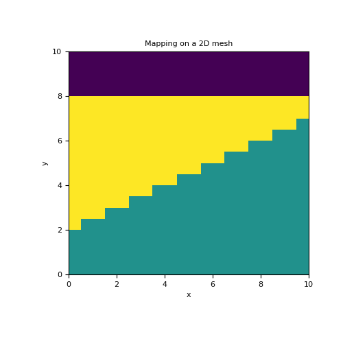
In this example, we define a 2 layer model whose interface is sharp and lies along a polynomial function \(y(x)=c_0 + c_1 x\). In this case, the model is defined as \(\mathbf{m} = [\sigma_1 , \sigma_2 , c_0 , c_1]\). We construct a polynomial mapping from the model to the set of active cells (i.e. below the surface), We then use an active cells mapping to map from the set of active cells to all cells in the 2D mesh.
>>> from SimPEG.maps import ParametricPolyMap, InjectActiveCells
>>> from discretize import TensorMesh
>>> import numpy as np
>>> import matplotlib.pyplot as plt
>>> h = 0.5*np.ones(20)
>>> mesh = TensorMesh([h, h])
>>> ind_active = mesh.cell_centers[:, 1] < 8
>>>
>>> sig1, sig2, c0, c1 = 10., 5., 2., 0.5
>>> model = np.r_[sig1, sig2, c0, c1]
>>> poly_map = ParametricPolyMap(
>>>     mesh, order=1, logSigma=False, normal='Y', actInd=ind_active, slope=1e4
>>> )
>>> act_map = InjectActiveCells(mesh, ind_active, 0.)
>>> fig = plt.figure(figsize=(5, 5))
>>> ax = fig.add_subplot(111)
>>> mesh.plot_image(act_map * poly_map * model, ax=ax)
>>> ax.set_title('Mapping on a 2D mesh')
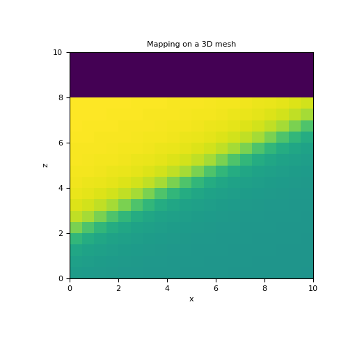
Here, we recreate the previous example on a 3D mesh but with a smoother interface. For a 3D mesh, the 2D polynomial defining the sloping interface is given by \(z(x,y) = c_0 + c_x x + c_y y + c_{xy} xy\). In this case, the model is defined as \(\mathbf{m} = [\sigma_1 , \sigma_2 , c_0 , c_x, c_y, c_{xy}]\).
>>> mesh = TensorMesh([h, h, h])
>>> ind_active = mesh.cell_centers[:, 2] < 8
>>>
>>> sig1, sig2, c0, cx, cy, cxy = 10., 5., 2., 0.5, 0., 0.
>>> model = np.r_[sig1, sig2, c0, cx, cy, cxy]
>>>
>>> poly_map = ParametricPolyMap(
>>>     mesh, order=[1, 1], logSigma=False, normal='Z', actInd=ind_active, slope=2
>>> )
>>> act_map = InjectActiveCells(mesh, ind_active, 0.)
>>>
>>> fig = plt.figure(figsize=(5, 5))
>>> ax = fig.add_subplot(111)
>>> mesh.plot_slice(act_map * poly_map * model, ax=ax, normal='Y', ind=10)
>>> ax.set_title('Mapping on a 3D mesh')

Attributes
Active indices of the mesh.
Determine whether or not this mapping is a linear operation.
Whether the input needs to be transformed by an exponential
The mesh used for the mapping
Number of active cells being mapped too.
Number of parameters the mapping acts on.
The projection axis.
Dimensions of the mapping.
Sharpness of the boundary.
Methods
deriv(m[, v])Derivative of the mapping with respect to the model.
dot(map1)Multiply two mappings to create a
SimPEG.maps.ComboMap.inverse(D)The transform inverse is not implemented.
test([m, num])Derivative test for the mapping.