Linear Least-Squares Inversion#

Here we demonstrate the basics of inverting data with SimPEG by considering a linear inverse problem. We formulate the inverse problem as a least-squares optimization problem. For this tutorial, we focus on the following:

Defining the forward problem

Defining the inverse problem (data misfit, regularization, optimization)

Specifying directives for the inversion

Recovering a set of model parameters which explains the observations

Import Modules#

import numpy as np
import matplotlib.pyplot as plt

from discretize import TensorMesh

from simpeg import (
    simulation,
    maps,
    data_misfit,
    directives,
    optimization,
    regularization,
    inverse_problem,
    inversion,
)

# sphinx_gallery_thumbnail_number = 3

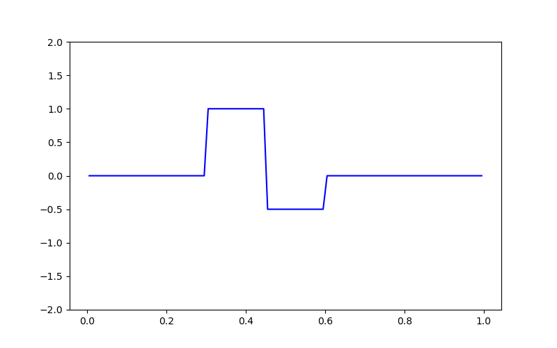
Defining the Model and Mapping#

Here we generate a synthetic model and a mappig which goes from the model space to the row space of our linear operator.

nParam = 100  # Number of model paramters

# A 1D mesh is used to define the row-space of the linear operator.
mesh = TensorMesh([nParam])

# Creating the true model
true_model = np.zeros(mesh.nC)
true_model[mesh.cell_centers_x > 0.3] = 1.0
true_model[mesh.cell_centers_x > 0.45] = -0.5
true_model[mesh.cell_centers_x > 0.6] = 0

# Mapping from the model space to the row space of the linear operator
model_map = maps.IdentityMap(mesh)

# Plotting the true model
fig = plt.figure(figsize=(8, 5))
ax = fig.add_subplot(111)
ax.plot(mesh.cell_centers_x, true_model, "b-")
ax.set_ylim([-2, 2])

(-2.0, 2.0)

Defining the Linear Operator#

Here we define the linear operator with dimensions (nData, nParam). In practive, you may have a problem-specific linear operator which you would like to construct or load here.

# Number of data observations (rows)
nData = 20

# Create the linear operator for the tutorial. The columns of the linear operator
# represents a set of decaying and oscillating functions.
jk = np.linspace(1.0, 60.0, nData)
p = -0.25
q = 0.25


def g(k):
    return np.exp(p * jk[k] * mesh.cell_centers_x) * np.cos(
        np.pi * q * jk[k] * mesh.cell_centers_x
    )


G = np.empty((nData, nParam))

for i in range(nData):
    G[i, :] = g(i)

# Plot the columns of G
fig = plt.figure(figsize=(8, 5))
ax = fig.add_subplot(111)
for i in range(G.shape[0]):
    ax.plot(G[i, :])

ax.set_title("Columns of matrix G")

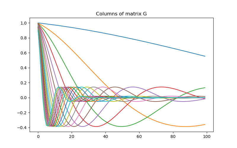
Text(0.5, 1.0, 'Columns of matrix G')

Defining the Simulation#

The simulation defines the relationship between the model parameters and predicted data.

sim = simulation.LinearSimulation(mesh, G=G, model_map=model_map)

Predict Synthetic Data#

Here, we use the true model to create synthetic data which we will subsequently invert.

# Standard deviation of Gaussian noise being added
std = 0.01
np.random.seed(1)

# Create a SimPEG data object
data_obj = sim.make_synthetic_data(true_model, relative_error=std, add_noise=True)

Define the Inverse Problem#

The inverse problem is defined by 3 things:

Data Misfit: a measure of how well our recovered model explains the field data

Regularization: constraints placed on the recovered model and a priori information

Optimization: the numerical approach used to solve the inverse problem

# Define the data misfit. Here the data misfit is the L2 norm of the weighted
# residual between the observed data and the data predicted for a given model.
# Within the data misfit, the residual between predicted and observed data are
# normalized by the data's standard deviation.
dmis = data_misfit.L2DataMisfit(simulation=sim, data=data_obj)

# Define the regularization (model objective function).
reg = regularization.WeightedLeastSquares(mesh, alpha_s=1.0, alpha_x=1.0)

# Define how the optimization problem is solved.
opt = optimization.InexactGaussNewton(maxIter=50)

# Here we define the inverse problem that is to be solved
inv_prob = inverse_problem.BaseInvProblem(dmis, reg, opt)

Define Inversion Directives#

Here we define any directiveas that are carried out during the inversion. This includes the cooling schedule for the trade-off parameter (beta), stopping criteria for the inversion and saving inversion results at each iteration.

# Defining a starting value for the trade-off parameter (beta) between the data
# misfit and the regularization.
starting_beta = directives.BetaEstimate_ByEig(beta0_ratio=1e-4)

# Setting a stopping criteria for the inversion.
target_misfit = directives.TargetMisfit()

# The directives are defined as a list.
directives_list = [starting_beta, target_misfit]

Setting a Starting Model and Running the Inversion#

To define the inversion object, we need to define the inversion problem and the set of directives. We can then run the inversion.

# Here we combine the inverse problem and the set of directives
inv = inversion.BaseInversion(inv_prob, directives_list)

# Starting model
starting_model = np.zeros(nParam)

# Run inversion
recovered_model = inv.run(starting_model)

Running inversion with SimPEG v0.24.1.dev37+gf5e5be547
============================ Inexact Gauss Newton ============================
  #     beta     phi_d     phi_m       f      |proj(x-g)-x|  LS    Comment
-----------------------------------------------------------------------------
1.82e+02  2.00e+05  0.00e+00  2.00e+05
1.82e+02  9.34e+04  7.02e-01  9.35e+04    2.50e+06      0
1.82e+02  6.38e+04  2.62e+00  6.42e+04    1.65e+05      0
1.82e+02  3.70e+04  9.45e+00  3.88e+04    1.22e+05      0   Skip BFGS
1.82e+02  2.50e+04  9.41e+00  2.67e+04    9.75e+04      0
1.82e+02  1.75e+04  1.49e+01  2.02e+04    1.53e+05      0
1.82e+02  8.67e+03  2.35e+01  1.29e+04    7.79e+04      0
1.82e+02  6.64e+03  2.40e+01  1.10e+04    9.12e+04      0
1.82e+02  5.57e+03  2.56e+01  1.02e+04    4.40e+04      0
1.82e+02  4.68e+03  2.70e+01  9.57e+03    1.52e+05      0
1.82e+02  2.74e+03  3.14e+01  8.45e+03    1.02e+05      0
1.82e+02  2.52e+03  3.20e+01  8.32e+03    9.00e+04      0
1.82e+02  2.05e+03  3.35e+01  8.13e+03    1.04e+05      0   Skip BFGS
1.82e+02  2.10e+03  3.26e+01  8.01e+03    1.10e+05      0
1.82e+02  2.03e+03  3.22e+01  7.88e+03    1.06e+05      0
1.82e+02  1.63e+03  3.26e+01  7.55e+03    1.05e+05      0   Skip BFGS
1.82e+02  1.47e+03  3.25e+01  7.38e+03    1.81e+04      0
1.82e+02  1.31e+03  3.32e+01  7.33e+03    2.63e+04      0   Skip BFGS
1.82e+02  1.25e+03  3.34e+01  7.31e+03    1.90e+04      0
1.82e+02  1.18e+03  3.37e+01  7.29e+03    2.30e+04      0   Skip BFGS
1.82e+02  1.18e+03  3.36e+01  7.28e+03    2.22e+04      0
1.82e+02  1.05e+03  3.42e+01  7.26e+03    2.69e+04      0   Skip BFGS
1.82e+02  1.10e+03  3.38e+01  7.24e+03    3.17e+04      0
1.82e+02  1.05e+03  3.41e+01  7.24e+03    3.69e+04      0   Skip BFGS
1.82e+02  1.06e+03  3.40e+01  7.23e+03    3.56e+04      0
1.82e+02  1.09e+03  3.38e+01  7.23e+03    3.26e+04      0   Skip BFGS
1.82e+02  1.06e+03  3.40e+01  7.23e+03    3.36e+04      0
1.82e+02  1.05e+03  3.40e+01  7.23e+03    3.23e+04      0   Skip BFGS
1.82e+02  1.06e+03  3.40e+01  7.23e+03    3.21e+04      0
1.82e+02  1.06e+03  3.39e+01  7.23e+03    3.25e+04      0   Skip BFGS
1.82e+02  1.06e+03  3.40e+01  7.23e+03    3.22e+04      0
1.82e+02  1.01e+03  3.38e+01  7.15e+03    3.30e+04      0   Skip BFGS
1.82e+02  1.02e+03  3.38e+01  7.15e+03    1.14e+04      0
1.82e+02  1.02e+03  3.38e+01  7.15e+03    1.37e+04      0   Skip BFGS
1.82e+02  1.01e+03  3.38e+01  7.14e+03    1.66e+04      0
1.82e+02  9.45e+02  3.41e+01  7.14e+03    1.53e+04      0   Skip BFGS
1.82e+02  9.47e+02  3.41e+01  7.14e+03    7.81e+03      0
1.82e+02  9.62e+02  3.40e+01  7.14e+03    7.97e+03      0
1.82e+02  9.61e+02  3.40e+01  7.14e+03    4.75e+03      0   Skip BFGS
1.82e+02  9.56e+02  3.41e+01  7.14e+03    4.47e+03      0
1.82e+02  9.51e+02  3.41e+01  7.14e+03    4.19e+03      0   Skip BFGS
1.82e+02  9.50e+02  3.41e+01  7.14e+03    3.92e+03      0
1.82e+02  9.48e+02  3.41e+01  7.14e+03    3.89e+03      0   Skip BFGS
1.82e+02  9.48e+02  3.41e+01  7.14e+03    2.88e+03      0
1.82e+02  9.48e+02  3.41e+01  7.14e+03    2.93e+03      0
1.82e+02  9.49e+02  3.41e+01  7.14e+03    2.93e+03      0   Skip BFGS
1.82e+02  9.50e+02  3.41e+01  7.14e+03    2.75e+03      0
1.82e+02  9.51e+02  3.41e+01  7.14e+03    3.34e+03      0   Skip BFGS
1.82e+02  9.51e+02  3.41e+01  7.14e+03    2.83e+03      0
1.82e+02  9.52e+02  3.41e+01  7.14e+03    2.89e+03      0   Skip BFGS
1.82e+02  9.51e+02  3.41e+01  7.14e+03    8.27e+03      0
------------------------- STOP! -------------------------
: |fc-fOld| = 2.6001e-02 <= tolF*(1+|f0|) = 2.0000e+04
: |xc-x_last| = 2.0397e-03 <= tolX*(1+|x0|) = 1.0000e-01
: |proj(x-g)-x|    = 2.5601e+03 <= tolG          = 1.0000e-01
: |proj(x-g)-x|    = 2.5601e+03 <= 1e3*eps       = 1.0000e-02
: maxIter   =      50    <= iter          =     50
------------------------- DONE! -------------------------

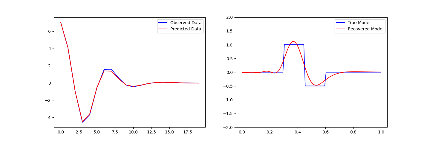
Plotting Results#

# Observed versus predicted data
fig, ax = plt.subplots(1, 2, figsize=(12 * 1.2, 4 * 1.2))
ax[0].plot(data_obj.dobs, "b-")
ax[0].plot(inv_prob.dpred, "r-")
ax[0].legend(("Observed Data", "Predicted Data"))

# True versus recovered model
ax[1].plot(mesh.cell_centers_x, true_model, "b-")
ax[1].plot(mesh.cell_centers_x, recovered_model, "r-")
ax[1].legend(("True Model", "Recovered Model"))
ax[1].set_ylim([-2, 2])