1D Forward Simulation with User-Defined Waveforms

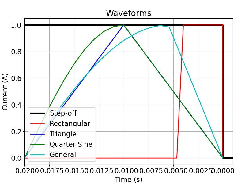
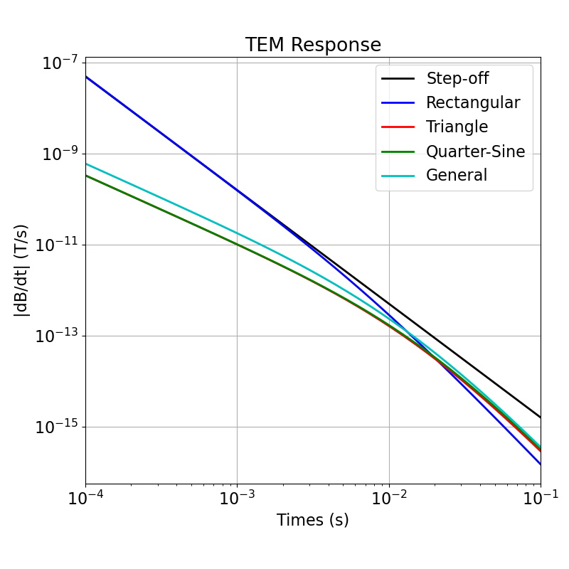
For time-domain electromagnetic problems, the response depends strongly on the souce waveforms. In this tutorial, we construct a set of waveforms of different types and simulate the response for a halfspace. Many types of waveforms can be constructed within SimPEG.electromagnetics.time_domain_1d. These include:

• the unit step off waveform

• a set of basic waveforms: rectangular, triangular, quarter sine, etc…

• a set of system-specific waveforms: SkyTEM, VTEM, GeoTEM, etc…

• fully customized waveforms

Import Modules

import numpy as np
import matplotlib as mpl
from matplotlib import pyplot as plt

mpl.rcParams.update({"font.size": 16})

from SimPEG import maps
import SimPEG.electromagnetics.time_domain as tdem

Define Waveforms

Here, we define the set of waveforms that will be used to simulated the TEM response.

# Unit stepoff waveform can be defined directly
stepoff_waveform = tdem.sources.StepOffWaveform()

# Rectangular waveform. The user may customize the waveform by setting the start
# time, end time and on time amplitude for the current waveform.
eps = 1e-6
ramp_on = np.r_[-0.004, -0.004 + eps]
ramp_off = np.r_[-eps, 0.0]
rectangular_waveform = tdem.sources.TrapezoidWaveform(
    ramp_on=ramp_on, ramp_off=ramp_off
)

# Triangular waveform. The user may customize the waveform by setting the start
# time, peak time, end time and peak amplitude for the current waveform.
eps = 1e-8
start_time = -0.02
peak_time = -0.01
off_time = 0.0
triangle_waveform = tdem.sources.TriangularWaveform(
    start_time=start_time, peak_time=peak_time, off_time=off_time
)

# Quarter-sine ramp-off
ramp_on = np.r_[-0.02, -0.01]
ramp_off = np.r_[-0.01, 0.0]
qs_waveform = tdem.sources.QuarterSineRampOnWaveform(ramp_on=ramp_on, ramp_off=ramp_off)


# General waveform. This is a fully general way to define the waveform.
# The use simply provides times and the current.
def custom_waveform(t, tmax):
    out = np.cos(0.5 * np.pi * (t - tmax) / (tmax + 0.02))
    out[t >= tmax] = 1 + (t[t >= tmax] - tmax) / tmax
    return out


waveform_times = np.r_[np.linspace(-0.02, -0.011, 10), -np.logspace(-2, -6, 61), 0.0]
waveform_current = custom_waveform(waveform_times, -0.0055)
general_waveform = tdem.sources.PiecewiseLinearWaveform(
    times=waveform_times, currents=waveform_current
)

Plot the Waveforms

Here, we plot the set of waveforms that are used in the simulation.

fig = plt.figure(figsize=(8, 6))
ax = fig.add_axes([0.1, 0.1, 0.85, 0.8])

ax.plot(np.r_[-2e-2, 0.0, 1e-10, 1e-3], np.r_[1.0, 1.0, 0.0, 0.0], "k", lw=3)
plotting_current = [rectangular_waveform.eval(t) for t in waveform_times]
ax.plot(waveform_times, plotting_current, "r", lw=2)
plotting_current = [triangle_waveform.eval(t) for t in waveform_times]
ax.plot(waveform_times, plotting_current, "b", lw=2)
plotting_current = [qs_waveform.eval(t) for t in waveform_times]
ax.plot(waveform_times, plotting_current, "g", lw=2)
plotting_current = [general_waveform.eval(t) for t in waveform_times]
ax.plot(waveform_times, plotting_current, "c", lw=2)

ax.grid()
ax.set_xlim([waveform_times.min(), 1e-3])
ax.set_xlabel("Time (s)")
ax.set_ylabel("Current (A)")
ax.set_title("Waveforms")
ax.legend(
    ["Step-off", "Rectangular", "Triangle", "Quarter-Sine", "General"], loc="lower left"
)

<matplotlib.legend.Legend object at 0x7f44aa61f730>

Create Survey

The waveform is a property of the source. So for each waveform, we will need to define a separate source object. For simplicity, all sources will be horizontal loops with a radius of 10 m.

# Define a receiver list. In this case, we measure the vertical component of
# db/dt. Thus we only have a single receiver in the list.
receiver_location = np.array([0.0, 0.0, 0.0])
receiver_orientation = "z"  # "x", "y" or "z"
times = np.logspace(-4, -1, 41)  # time channels

receiver_list = [
    tdem.receivers.PointMagneticFluxTimeDerivative(
        receiver_location, times, orientation=receiver_orientation
    )
]

# Source properties. If you defined the true waveform (not normalized), the current amplitude
# should be set to 1. Otherwise you will be accounting for the maximum current
# amplitude twice!!!
source_location = np.array([0.0, 0.0, 0.0])
source_radius = 10.0
current_amplitude = 1.0

source_list = []

# Stepoff Waveform
source_list.append(
    tdem.sources.CircularLoop(
        receiver_list=receiver_list,
        location=source_location,
        waveform=stepoff_waveform,
        radius=source_radius,
        current=current_amplitude,
    )
)

# Rectangular Waveform
source_list.append(
    tdem.sources.CircularLoop(
        receiver_list=receiver_list,
        location=source_location,
        waveform=rectangular_waveform,
        radius=source_radius,
        current=current_amplitude,
    )
)

# Triangle Waveform
source_list.append(
    tdem.sources.CircularLoop(
        receiver_list=receiver_list,
        location=source_location,
        waveform=triangle_waveform,
        radius=source_radius,
        current=current_amplitude,
    )
)

# Quarter-sine ramp-off Waveform
source_list.append(
    tdem.sources.CircularLoop(
        receiver_list=receiver_list,
        location=source_location,
        waveform=qs_waveform,
        radius=source_radius,
        current=current_amplitude,
    )
)

# General Waveform
source_list.append(
    tdem.sources.CircularLoop(
        receiver_list=receiver_list,
        location=source_location,
        waveform=general_waveform,
        radius=source_radius,
        current=current_amplitude,
    )
)

# Survey
survey = tdem.Survey(source_list)

Defining a 1D Layered Earth Model

Here, we define the layer thicknesses and electrical conductivities for our 1D simulation. If we have N layers, we define N electrical conductivity values and N-1 layer thicknesses. The lowest layer is assumed to extend to infinity.

# Layer thicknesses
thicknesses = np.array([40.0, 40.0])
n_layer = len(thicknesses) + 1

# half-space physical properties
sigma = 1e-2
eta = 0.5
tau = 0.01
c = 0.5
chi = 0.0

# physical property models
sigma_model = sigma * np.ones(n_layer)
eta_model = eta * np.ones(n_layer)
tau_model = tau * np.ones(n_layer)
c_model = c * np.ones(n_layer)
mu0 = 4 * np.pi * 1e-7
mu_model = mu0 * (1 + chi) * np.ones(n_layer)

# Define a mapping for conductivities
model_mapping = maps.IdentityMap(nP=n_layer)

Define the Forward Simulation and Predict Data

# Define the simulation
simulation = tdem.Simulation1DLayered(
    survey=survey, thicknesses=thicknesses, sigmaMap=model_mapping, mu=mu_model
)

# Predict data for a given model
dpred = simulation.dpred(sigma_model)

Plotting Results

fig = plt.figure(figsize=(8, 8))
d = np.reshape(dpred, (len(source_list), len(times))).T
ax = fig.add_axes([0.15, 0.15, 0.8, 0.75])
colorlist = ["k", "b", "r", "g", "c"]
for ii, k in enumerate(colorlist):
    ax.loglog(times, np.abs(d[:, ii]), k, lw=2)

ax.set_xlim([times.min(), times.max()])
ax.grid()
ax.legend(["Step-off", "Rectangular", "Triangle", "Quarter-Sine", "General"])
ax.set_xlabel("Times (s)")
ax.set_ylabel("|dB/dt| (T/s)")
ax.set_title("TEM Response")

Text(0.5, 1.0, 'TEM Response')

Estimated memory usage: 8 MB