simpeg.regularization.PGI#

class simpeg.regularization.PGI(mesh, gmmref, alpha_x=None, alpha_y=None, alpha_z=None, alpha_xx=0.0, alpha_yy=0.0, alpha_zz=0.0, gmm=None, wiresmap=None, maplist=None, alpha_pgi=1.0, approx_hessian=True, approx_gradient=True, approx_eval=True, weights_list=None, non_linear_relationships=False, reference_model_in_smooth=False, **kwargs)[source]#

Bases: ComboObjectiveFunction

Regularization function for petrophysically guided inversion (PGI).

PGI is used to recover models in which 1) the physical property values are consistent with petrophysical information and 2) structures in the recovered model are geologically plausible. PGI regularization is a weighted sum of PGIsmallness, SmoothnessFirstOrder and SmoothnessSecondOrder (optional) regularization functions. The PGI smallness term assumes the statistical distribution of physical property values defining the model is characterized by a Gaussian mixture model (GMM). And the smoothness terms penalize large spatial derivatives in the recovered model.

PGI can be implemented to invert for a single physical property or multiple physical properties, each of which are defined on a linear scale (e.g. density) or a log-scale (e.g. electrical conductivity). If the statistical distribution(s) of physical property values for each property type are known, the GMM can be constructed and left static throughout the inversion. Otherwise, the recovered model at each iteration is used to update the GMM. And the updated GMM is used to constrain the recovered model for the following iteration.

Parameters:

meshsimpeg.regularization.RegularizationMesh, discretize.base.BaseMesh: Mesh on which the regularization is discretized. Implemented for tensor, QuadTree or Octree meshes.
gmmrefsimpeg.utils.WeightedGaussianMixture: Reference Gaussian mixture model.
gmmNone, simpeg.utils.WeightedGaussianMixture: Set the Gaussian mixture model used to constrain the recovered physical property model. Can be left static throughout the inversion or updated using the directives.PGI_UpdateParameters directive. If None, the directives.PGI_UpdateParameters directive must be used to ensure there is a Gaussian mixture model for the inversion.
alpha_pgifloat: Scaling constant for the PGI smallness term.
alpha_x, alpha_y, alpha_zfloat or None, optional: Scaling constants for the first order smoothness along x, y and z, respectively. If set to None, the scaling constant is set automatically according to the value of the length_scale parameter.
alpha_xx, alpha_yy, alpha_zz0, float: Scaling constants for the second order smoothness along x, y and z, respectively. If set to None, the scaling constant is set automatically according to the length scales; see regularization.WeightedLeastSquares.
wiresmapNone, simpeg.maps.Wires: Mapping from the model to the model parameters of each type. If None, we assume only a single physical property type in the inversion.
maplistNone, list of simpeg.maps: Ordered list of mappings from model values to physical property values; one for each physical property. If None, we assume a single physical property type in the regularization and an maps.IdentityMap from model values to physical property values.
approx_gradientbool: If True, use the L2-approximation of the gradient by assuming physical property values of different types are uncorrelated.
approx_evalbool: If True, use the L2-approximation evaluation of the smallness term by assuming physical property values of different types are uncorrelated.
approx_hessianbool: Approximate the Hessian of the regularization function.
non_linear_relationshipbool: Whether relationships in the Gaussian mixture model are non-linear.
reference_model_in_smoothbool, optional: Whether to include the reference model in the smoothness terms.

Attributes

`W`	Full weighting matrix for the combo objective function.
`alpha_pgi`	Scaling constant for the PGI smallness term.
`gmm`	Gaussian mixture model.
`maplist`	Ordered list of mappings from model values to physical property values.
`mapping`	Mapping from the model to the quantity evaluated in the object function.
`multipliers`	Multipliers for the objective functions.
`nP`	Number of model parameters.
`reference_model`	Reference model.
`reference_model_in_smooth`	Whether to include the reference model in the smoothness objective functions.
`regularization_mesh`	Regularization mesh.
`wiresmap`	Mapping from the model to the model parameters of each type.

Methods

`__call__`(m[, f])	Evaluate the objective functions for a given model.
`compute_quasi_geology_model`()	Compute and return quasi geology model.
`deriv`(m[, f])	Gradient of the objective function evaluated for the model provided.
`deriv2`(m[, v, f])	Hessian of the objective function evaluated for the model provided.
`get_functions_of_type`(fun_class)	Return objective functions of a given type(s).
`map_class`	alias of `IdentityMap`
`membership`(m)	Compute and return membership array for the model provided.
`test`([x, num, random_seed])	Run a convergence test on both the first and second derivatives.

Notes

For one or more physical property types (e.g. conductivity, density, susceptibility), the PGI regularization function (objective function) is derived by using a Gaussian mixture model (GMM) to construct the prior within a Baysian inversion scheme. For a comprehensive description, see (Astic, et al 2019; Astic et al 2020).

We let \(\Theta\) store all of the means (\(\boldsymbol{\mu}\)), covariances (\(\boldsymbol{\Sigma}\)) and proportion constants (\(\boldsymbol{\gamma}\)) defining the GMM. And let \(\mathbf{z}^\ast\) define an membership array that extracts the GMM parameters for the most representative rock unit within each active cell in the RegularizationMesh. The regularization function (objective function) for PGI is given by:

\[\begin{split}\phi (\mathbf{m}) &= \alpha_\text{pgi} \big [ \mathbf{m} - \mathbf{m_{ref}}(\Theta, \mathbf{z}^\ast ) \big ]^T \mathbf{W} ( \Theta , \mathbf{z}^\ast ) \, \big [ \mathbf{m} - \mathbf{m_{ref}}(\Theta, \mathbf{z}^\ast ) \big ] \\ &+ \sum_{j=x,y,z} \alpha_j \Big \| \mathbf{W_j G_j \, m} \, \Big \|^2 \\ &+ \sum_{j=x,y,z} \alpha_{jj} \Big \| \mathbf{W_{jj} L_j \, m} \, \Big \|^2 \;\;\;\;\;\;\;\; \big ( \textrm{optional} \big )\end{split}\]

where

\(\mathbf{m}\) is the model,

\(\mathbf{m_{ref}}(\Theta, \mathbf{z}^\ast )\) is the reference model,

\(\mathbf{G_x, \, G_y, \; G_z}\) are partial cell gradients operators along x, y and z,

\(\mathbf{L_x, \, L_y, \; L_z}\) are second-order derivative operators with respect to x, y and z,

\(\mathbf{W}(\Theta , \mathbf{z}^\ast )\) is the weighting matrix for PGI smallness, and

\(\mathbf{W_x, \, W_y, \; W_z}\) are weighting matrices for smoothness terms.

PGIsmallness regularization can be used for models consisting of one or more physical property types. The ordering of the physical property types within the model is defined using the wiresmap. And the mapping from model parameter values to physical property values is specified with maplist. For \(K\) physical property types, the model is an array vector of the form:

\[\begin{split}\mathbf{m} = \begin{bmatrix} \mathbf{m}_1 \\ \mathbf{m}_2 \\ \vdots \\ \mathbf{m}_K \end{bmatrix}\end{split}\]

When the approx_eval property is True, we assume the physical property types have values that are uncorrelated. In this case, the weighting matrix is diagonal and the regularization function (objective function) can be expressed as:

\[\begin{split}\phi (\mathbf{m}) &= \alpha_\text{pgi} \Big \| \mathbf{W}_{\! 1/2}(\Theta, \mathbf{z}^\ast ) \, \big [ \mathbf{m} - \mathbf{m_{ref}}(\Theta, \mathbf{z}^\ast ) \big ] \, \Big \|^2 \\ &+ \sum_{j=x,y,z} \alpha_j \Big \| \mathbf{W_j G_j \, m} \, \Big \|^2 \\ &+ \sum_{j=x,y,z} \alpha_{jj} \Big \| \mathbf{W_{jj} L_j \, m} \, \Big \|^2 \;\;\;\;\;\;\;\; \big ( \textrm{optional} \big )\end{split}\]

When the approx_eval property is True, you may also set the approx_gradient property to True so that the least-squares approximation is used to compute the gradient.

Constructing the Reference Model and Weighting Matrix:

The reference model used in the regularization function is constructed by extracting the means \(\boldsymbol{\mu}\) from the GMM using the membership array \(\mathbf{z}^\ast\). We represent this vector as:

\[\mathbf{m_{ref}} (\Theta ,{\mathbf{z}^\ast}) = \boldsymbol{\mu}_{\mathbf{z}^\ast}\]

To construct the weighting matrix, \(\mathbf{z}^\ast\) is used to extract the covariances \(\boldsymbol{\Sigma}\) for each cell. And the weighting matrix is given by:

\[\mathbf{W}(\Theta ,{\mathbf{z}^\ast } ) = \boldsymbol{\Sigma}_{\mathbf{z^\ast}}^{-1} \, diag \big ( \mathbf{v \odot w} \big )\]

where \(\mathbf{v}\) are the volumes of the active cells, and \(\mathbf{w}\) are custom cell weights. When the approx_eval property is True, the off-diagonal covariances are zero and we can use a weighting matrix of the form:

\[\mathbf{W}_{\! 1/2}(\Theta ,{\mathbf{z}^\ast } ) = diag \Big ( \big [ \mathbf{v \odot w} \odot \boldsymbol{\sigma}_{\mathbf{z}^\ast}^{-2} \big ]^{1/2} \Big )\]

where \(\boldsymbol{\sigma}_{\mathbf{z}^\ast}^2\) are the variances extracted using the membership array \(\mathbf{z}^\ast\).

Updating the Gaussian Mixture Model:

When the GMM is set using the gmm property, the GMM remains static throughout the inversion. When the gmm property set as None, the GMM is learned and updated after every model update. That is, we assume the GMM defined using the gmmref property is not completely representative of the physical property distributions for each rock unit, and we update the all of the means (\(\boldsymbol{\mu}\)), covariances (\(\boldsymbol{\Sigma}\)) and proportion constants (\(\boldsymbol{\gamma}\)) defining the GMM \(\Theta\). This is done by solving:

\[\max_\Theta \; \mathcal{P}(\Theta | \mathbf{m})\]

using a MAP variation of the expectation-maximization clustering algorithm introduced in Dempster (et al. 1977).

Updating the Membership Array:

As the model (and GMM) are updated throughout the inversion, the rock unit considered most indicative of the geology within each cell is updated; which is represented by the membership array \(\mathbf{z}^\ast\). W. For the current GMM with means (\(\boldsymbol{\mu}\)), covariances (\(\boldsymbol{\Sigma}\)) and proportion constants (\(\boldsymbol{\gamma}\)), we solve the following for each cell:

\[z_i^\ast = \max_n \; \gamma_{i,n} \, \mathcal{N} (\mathbf{m}_i | \boldsymbol{\mu}_n , \boldsymbol{\Sigma}_n)\]

where

\(\mathbf{m_i}\) are the model values for cell \(i\),

\(\gamma_{i,n}\) is the proportion for cell \(i\) and rock unit \(n\)

\(\boldsymbol{\mu}_n\) are the mean property values for unit \(n\),

\(\boldsymbol{\Sigma}_n\) are the covariances for unit \(n\), and

\(\mathcal{N}\) represent the multivariate Gaussian distribution.

Galleries and Tutorials using `simpeg.regularization.PGI`#

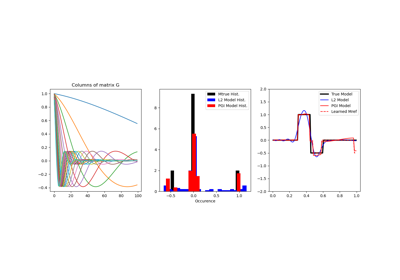
Petrophysically guided inversion (PGI): Linear example

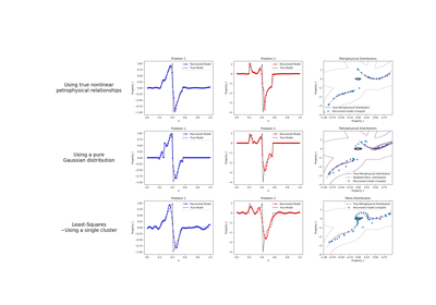
Petrophysically guided inversion: Joint linear example with nonlinear relationships

Joint PGI of Gravity + Magnetic on an Octree mesh using full petrophysical information

Joint PGI of Gravity + Magnetic on an Octree mesh without petrophysical information

simpeg.regularization.PGI#

Galleries and Tutorials using simpeg.regularization.PGI#

This Page

Galleries and Tutorials using `simpeg.regularization.PGI`#