Magnetic inversion on a TreeMesh

In this example, we demonstrate the use of a Magnetic Vector Inversion on 3D TreeMesh for the inversion of magnetic data.

The inverse problem uses the simpeg.regularization.VectorAmplitude regularization.

from simpeg import (
    data,
    data_misfit,
    directives,
    maps,
    inverse_problem,
    optimization,
    inversion,
    regularization,
)

from simpeg import utils
from simpeg.utils import mkvc, sdiag

from discretize.utils import mesh_builder_xyz, active_from_xyz
from simpeg.potential_fields import magnetics
import numpy as np
import matplotlib.pyplot as plt

# sphinx_gallery_thumbnail_number = 3

Setup

Define the survey and model parameters

First we need to define the direction of the inducing field As a simple case, we pick a vertical inducing field of magnitude 50,000 nT.

np.random.seed(1)
# We will assume a vertical inducing field
h0_amplitude, h0_inclination, h0_declination = (50000.0, 90.0, 0.0)

# Create grid of points for topography
# Lets create a simple Gaussian topo and set the active cells
[xx, yy] = np.meshgrid(np.linspace(-200, 200, 50), np.linspace(-200, 200, 50))
b = 100
A = 50
zz = A * np.exp(-0.5 * ((xx / b) ** 2.0 + (yy / b) ** 2.0))
topo = np.c_[utils.mkvc(xx), utils.mkvc(yy), utils.mkvc(zz)]

# Create an array of observation points
xr = np.linspace(-100.0, 100.0, 20)
yr = np.linspace(-100.0, 100.0, 20)
X, Y = np.meshgrid(xr, yr)
Z = A * np.exp(-0.5 * ((X / b) ** 2.0 + (Y / b) ** 2.0)) + 5

# Create a MAGsurvey
xyzLoc = np.c_[mkvc(X.T), mkvc(Y.T), mkvc(Z.T)]
rxLoc = magnetics.receivers.Point(xyzLoc)
srcField = magnetics.sources.UniformBackgroundField(
    receiver_list=[rxLoc],
    amplitude=h0_amplitude,
    inclination=h0_inclination,
    declination=h0_declination,
)
survey = magnetics.survey.Survey(srcField)

Inversion Mesh

Here, we create a TreeMesh with base cell size of 5 m.

# Create a mesh
h = [5, 5, 5]
padDist = np.ones((3, 2)) * 100

mesh = mesh_builder_xyz(
    xyzLoc, h, padding_distance=padDist, depth_core=100, mesh_type="tree"
)
mesh.refine_surface(topo, level=-1, padding_cells_by_level=[3, 3], finalize=True)


# Define an active cells from topo
actv = active_from_xyz(mesh, topo)
nC = int(actv.sum())

/usr/share/miniconda/envs/simpeg-test/lib/python3.12/site-packages/discretize/utils/mesh_utils.py:528: FutureWarning: In discretize v1.0 the TreeMesh will change the default value of diagonal_balance to True, which will likely slightly change meshes you have previously created. If you need to keep the current behavior, explicitly set diagonal_balance=False.
  mesh = discretize.TreeMesh(h_dim, diagonal_balance=tree_diagonal_balance)
/home/vsts/work/1/s/examples/03-magnetics/plot_inv_mag_MVI_VectorAmplitude.py:87: FutureWarning: In discretize v1.0 refine_surface will change the default behavior of horizontal padding to extrapolate the surface outwards from the nodes on its boundary, instead of stretching its bounding box. To use the new behavior now, set extrapolate_surface=True. To keep the current behavior, explicitly set extrapolate_surface=False.
  mesh.refine_surface(topo, level=-1, padding_cells_by_level=[3, 3], finalize=True)

Forward modeling data

We can now create a magnetization model and generate data.

model_azm_dip = np.zeros((mesh.nC, 2))
model_amp = np.ones(mesh.nC) * 1e-8
ind = utils.model_builder.get_indices_block(
    np.r_[-30, -20, -10],
    np.r_[30, 20, 25],
    mesh.gridCC,
)
model_amp[ind] = 0.05
model_azm_dip[ind, 0] = 45.0
model_azm_dip[ind, 1] = 90.0

# Remove air cells
model_azm_dip = model_azm_dip[actv, :]
model_amp = model_amp[actv]
model = sdiag(model_amp) * utils.mat_utils.dip_azimuth2cartesian(
    model_azm_dip[:, 0], model_azm_dip[:, 1]
)

# Create reduced identity map
idenMap = maps.IdentityMap(nP=nC * 3)

# Create the simulation
simulation = magnetics.simulation.Simulation3DIntegral(
    survey=survey, mesh=mesh, chiMap=idenMap, active_cells=actv, model_type="vector"
)

# Compute some data and add some random noise
d = simulation.dpred(mkvc(model))
std = 10  # nT
synthetic_data = d + np.random.randn(len(d)) * std
wd = np.ones(len(d)) * std

# Assign data and uncertainties to the survey
data_object = data.Data(survey, dobs=synthetic_data, standard_deviation=wd)

# Create a projection matrix for plotting later
actv_plot = maps.InjectActiveCells(mesh, actv, np.nan)

/home/vsts/work/1/s/examples/03-magnetics/plot_inv_mag_MVI_VectorAmplitude.py:102: BreakingChangeWarning: Since SimPEG v0.25.0, the 'get_indices_block' function returns a single array with the cell indices, instead of a tuple with a single element. This means that we don't need to unpack the tuple anymore to access to the cell indices.
If you were using this function as in:

    ind = get_indices_block(p0, p1, mesh.cell_centers)[0]

Make sure you update it to:

    ind = get_indices_block(p0, p1, mesh.cell_centers)

To hide this warning, add this to your script or notebook:

    import warnings
    from simpeg.utils import BreakingChangeWarning

    warnings.filterwarnings(action='ignore', category=BreakingChangeWarning)

  ind = utils.model_builder.get_indices_block(

Inversion

We can now attempt the inverse calculations.

# Create sensitivity weights from our linear forward operator
rxLoc = survey.source_field.receiver_list[0].locations

# This Mapping connects the regularizations for the three-component
# vector model
wires = maps.Wires(("p", nC), ("s", nC), ("t", nC))
m0 = np.ones(3 * nC) * 1e-4  # Starting model

# Create the regularization on the amplitude of magnetization
reg = regularization.VectorAmplitude(
    mesh,
    mapping=idenMap,
    active_cells=actv,
    reference_model_in_smooth=True,
    norms=[0.0, 2.0, 2.0, 2.0],
    gradient_type="total",
)

# Data misfit function
dmis = data_misfit.L2DataMisfit(simulation=simulation, data=data_object)
dmis.W = 1.0 / data_object.standard_deviation

# The optimization scheme
opt = optimization.ProjectedGNCG(
    maxIter=20, lower=-10, upper=10.0, maxIterLS=20, cg_maxiter=20, cg_rtol=1e-3
)

# The inverse problem
invProb = inverse_problem.BaseInvProblem(dmis, reg, opt)

# Estimate the initial beta factor
betaest = directives.BetaEstimate_ByEig(beta0_ratio=1e1)

# Add sensitivity weights
sensitivity_weights = directives.UpdateSensitivityWeights()

# Here is where the norms are applied
IRLS = directives.UpdateIRLS(
    f_min_change=1e-3, max_irls_iterations=10, misfit_tolerance=5e-1
)

# Pre-conditioner
update_Jacobi = directives.UpdatePreconditioner()


inv = inversion.BaseInversion(
    invProb, directiveList=[sensitivity_weights, IRLS, update_Jacobi, betaest]
)

# Run the inversion
mrec = inv.run(m0)

Running inversion with SimPEG v0.26.0
================================================= Projected GNCG =================================================
  #     beta     phi_d     phi_m       f      |proj(x-g)-x|  LS   iter_CG   CG |Ax-b|/|b|  CG |Ax-b|   Comment
-----------------------------------------------------------------------------------------------------------------
   0  2.56e+05  1.19e+04  0.00e+00  1.19e+04                         0           inf          inf
   1  2.56e+05  8.71e+03  5.58e-03  1.01e+04    2.69e+03      0      20       3.59e-01     9.50e+04
   2  1.28e+05  6.74e+03  1.63e-02  8.83e+03    2.22e+03      0      11       7.90e-04     1.02e+02
   3  6.39e+04  4.60e+03  4.06e-02  7.19e+03    2.05e+03      0      13       6.77e-04     5.11e+01
   4  3.20e+04  2.65e+03  8.40e-02  5.33e+03    1.96e+03      0      14       7.49e-04     4.32e+01
   5  1.60e+04  1.30e+03  1.43e-01  3.59e+03    1.84e+03      0      17       5.63e-04     2.28e+01
   6  7.99e+03  5.72e+02  2.06e-01  2.22e+03    1.71e+03      0      18       7.32e-04     1.93e+01
   7  3.99e+03  2.45e+02  2.62e-01  1.29e+03    1.56e+03      0      20       1.49e-03     2.41e+01
Reached starting chifact with l2-norm regularization: Start IRLS steps...
irls_threshold 0.008782292469391058
   8  3.99e+03  4.54e+02  3.74e-01  1.95e+03    1.64e+03      0      18       7.48e-04     1.34e+01
   9  3.99e+03  7.00e+02  4.61e-01  2.54e+03    1.64e+03      0      14       9.36e-04     1.72e+01
  10  2.64e+03  6.51e+02  6.67e-01  2.41e+03    1.32e+03      0      14       6.45e-04     5.05e+00
  11  1.80e+03  6.28e+02  9.14e-01  2.27e+03    1.62e+03      0      13       4.72e-04     7.59e+00
  12  1.25e+03  5.76e+02  1.11e+00  1.97e+03    1.66e+03      0      11       9.37e-04     1.84e+01
  13  1.25e+03  6.43e+02  1.06e+00  1.97e+03    1.79e+03      0      10       6.13e-04     1.84e+01
  14  8.56e+02  5.24e+02  1.12e+00  1.48e+03    9.76e+02      0      11       6.38e-04     4.42e+00
  15  8.56e+02  5.41e+02  1.07e+00  1.45e+03    1.51e+03      0      9        7.46e-04     8.37e+00
  16  8.56e+02  5.48e+02  1.03e+00  1.43e+03    1.40e+03      0      9        5.74e-04     4.75e+00
  17  8.56e+02  5.52e+02  1.00e+00  1.41e+03    1.37e+03      0      9        5.04e-04     4.17e+00
Reach maximum number of IRLS cycles: 10
------------------------- STOP! -------------------------
1 : |fc-fOld| = 1.8706e+01 <= tolF*(1+|f0|) = 1.1928e+03
1 : |xc-x_last| = 2.4438e-02 <= tolX*(1+|x0|) = 1.0360e-01
0 : |proj(x-g)-x|    = 1.3745e+03 <= tolG          = 1.0000e-01
0 : |proj(x-g)-x|    = 1.3745e+03 <= 1e3*eps       = 1.0000e-02
0 : maxIter   =      20    <= iter          =     17
------------------------- DONE! -------------------------

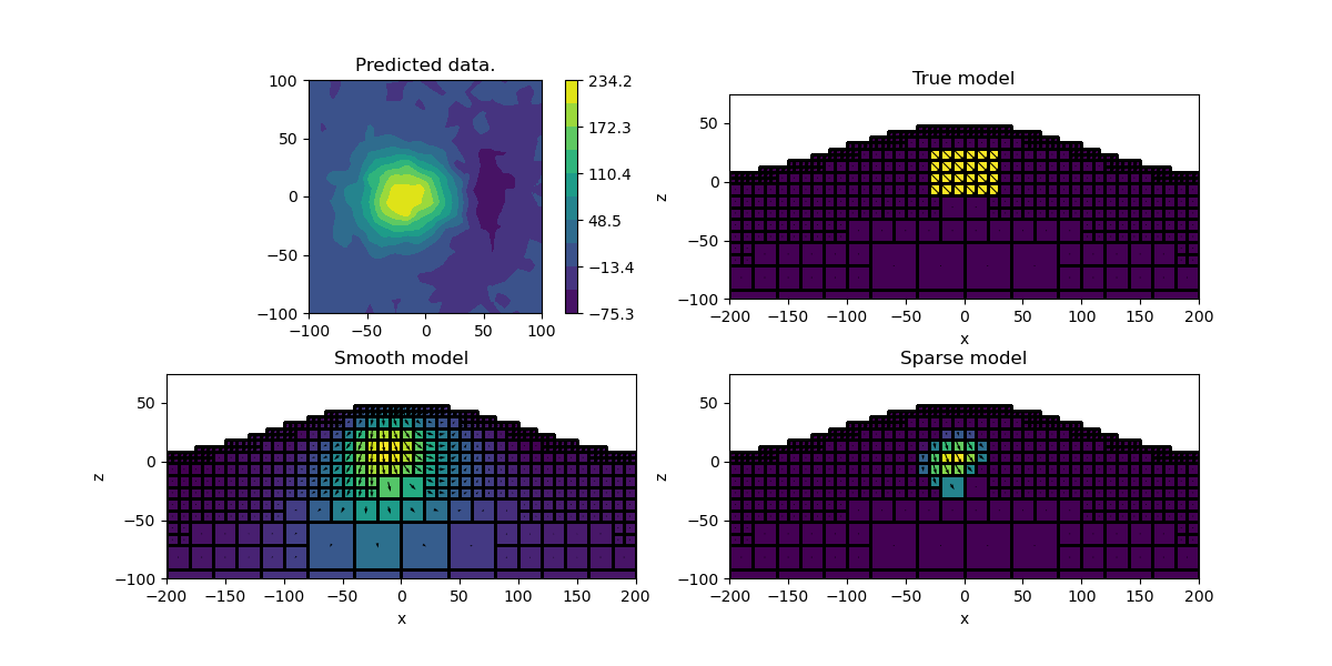
Final Plot

Let’s compare the smooth and compact model

plt.figure(figsize=(12, 6))
ax = plt.subplot(2, 2, 1)
im = utils.plot_utils.plot2Ddata(xyzLoc, synthetic_data, ax=ax)
plt.colorbar(im[0])
ax.set_title("Predicted data.")
plt.gca().set_aspect("equal", adjustable="box")

for ii, (title, mvec) in enumerate(
    [("True model", model), ("Smooth model", invProb.l2model), ("Sparse model", mrec)]
):
    ax = plt.subplot(2, 2, ii + 2)
    mesh.plot_slice(
        actv_plot * mvec.reshape((-1, 3), order="F"),
        v_type="CCv",
        view="vec",
        ax=ax,
        normal="Y",
        grid=True,
        quiver_opts={
            "pivot": "mid",
            "scale": 8 * np.abs(mvec).max(),
            "scale_units": "inches",
        },
    )
    ax.set_xlim([-200, 200])
    ax.set_ylim([-100, 75])
    ax.set_title(title)
    ax.set_xlabel("x")
    ax.set_ylabel("z")
    plt.gca().set_aspect("equal", adjustable="box")

plt.show()

# Plot the final predicted data and the residual
# plt.figure()
# ax = plt.subplot(1, 2, 1)
# utils.plot_utils.plot2Ddata(xyzLoc, invProb.dpred, ax=ax)
# ax.set_title("Predicted data.")
# plt.gca().set_aspect("equal", adjustable="box")
#
# ax = plt.subplot(1, 2, 2)
# utils.plot_utils.plot2Ddata(xyzLoc, synthetic_data - invProb.dpred, ax=ax)
# ax.set_title("Data residual.")
# plt.gca().set_aspect("equal", adjustable="box")

Estimated memory usage: 530 MB