simpeg.maps.SelfConsistentEffectiveMedium#
- class simpeg.maps.SelfConsistentEffectiveMedium(mesh=None, nP=None, sigma0=None, sigma1=None, alpha0=1.0, alpha1=1.0, orientation0='z', orientation1='z', random=True, rel_tol=0.001, maxIter=50, **kwargs)[source]#
Bases:
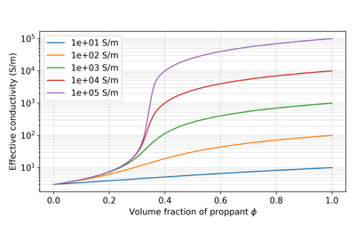
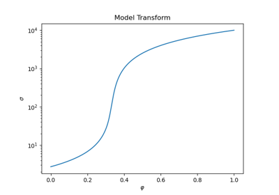
IdentityMapTwo phase self-consistent effective medium theory mapping for ellipsoidal inclusions. The inversion model is the concentration (volume fraction) of the phase 2 material.
The inversion model is \(\varphi\). We solve for \(\sigma\) given \(\sigma_0\), \(\sigma_1\) and \(\varphi\) . Each of the following are implicit expressions of the effective conductivity. They are solved using a fixed point iteration.
Spherical Inclusions
If the shape of the inclusions are spheres, we use
\[\sum_{j=1}^N (\sigma^* - \sigma_j)R^{j} = 0\]where \(j=[1,N]\) is the each material phase, and N is the number of phases. Currently, the implementation is only set up for 2 phase materials, so we solve
\[\begin{split}(1-\\varphi)(\sigma - \sigma_0)R^{(0)} + \varphi(\sigma - \sigma_1)R^{(1)} = 0.\end{split}\]Where \(R^{(j)}\) is given by
\[R^{(j)} = \left[1 + \frac{1}{3}\frac{\sigma_j - \sigma}{\sigma} \right]^{-1}.\]Ellipsoids
If the inclusions are aligned ellipsoids, we solve
\[\sum_{j=1}^N \varphi_j (\Sigma^* - \sigma_j\mathbf{I}) \mathbf{R}^{j, *} = 0\]where
\[\begin{split}\mathbf{R}^{(j, *)} = \left[ \mathbf{I} + \mathbf{A}_j {\Sigma^{*}}^{-1}(\sigma_j \mathbf{I} - \Sigma^*) \\right]^{-1}\end{split}\]and the depolarization tensor \(\mathbf{A}_j\) is given by
\[\begin{split}\mathbf{A}^* = \left[\begin{array}{ccc} Q & 0 & 0 \\ 0 & Q & 0 \\ 0 & 0 & 1-2Q \end{array}\right]\end{split}\]for a spheroid aligned along the z-axis. For an oblate spheroid (\(\alpha < 1\), pancake-like)
\[Q = \frac{1}{2}\left( 1 + \frac{1}{\alpha^2 - 1} \left[ 1 - \frac{1}{\chi}\tan^{-1}(\chi) \right] \right)\]where
\[\chi = \sqrt{\frac{1}{\alpha^2} - 1}\]For reference, see Torquato (2002), Random Heterogeneous Materials
Attributes
Aspect ratio of the phase-0 ellipsoids.
Aspect ratio of the phase-1 ellipsoids.
Determine whether or not this mapping is a linear operation.
Maximum number of iterations for the fixed point iteration calculation.
The mesh used for the mapping
Number of parameters the mapping acts on.
Orientation of the phase-0 inclusions.
Orientation of the phase-0 inclusions.
Are the inclusions randomly oriented (True) or preferentially aligned (False)?
relative tolerance for convergence for the fixed-point iteration.
Dimensions of the mapping operator
Physical property value for phase-0 material.
Physical property value for phase-1 material.
first guess for sigma
absolute tolerance for the convergence of the fixed point iteration calc
Methods
deriv(m[, v])Derivative of the effective conductivity with respect to the volume fraction of phase 2 material
dot(map1)Multiply two mappings to create a
simpeg.maps.ComboMap.getA(alpha, orientation)Depolarization tensor
getQ(alpha)Geometric factor in the depolarization tensor
getR(sj, se, alpha[, orientation])Electric field concentration tensor
getdR(sj, se, alpha[, orientation])Derivative of the electric field concentration tensor with respect to the concentration of the second phase material.
hashin_shtrikman_bounds(phi1)Hashin Shtrikman bounds
Hashin Shtrikman bounds for anisotropic media
inverse(sige)Compute the concentration given the effective conductivity
test([m, num, random_seed])Derivative test for the mapping.
wiener_bounds(phi1)Define Wenner Conductivity Bounds