Note
Go to the end to download the full example code
1D Forward Simulation for a Single Sounding#
Here we use the module SimPEG.electromangetics.time_domain_1d to predict the stepoff response for a single sounding over a 1D layered Earth. In this tutorial, we focus on the following:
Defining receivers, waveforms, sources and the survey
The units of the model and resulting data
Defining and running the 1D simulation for a single sounding
Our survey geometry consists of a horizontal loop source with a radius of 6 m located 20 m above the Earth’s surface. The receiver is located at the centre of the loop and measures the vertical component of the response.
Import Modules#
import numpy as np
import os
from matplotlib import pyplot as plt

from SimPEG import maps
import SimPEG.electromagnetics.time_domain as tdem
from SimPEG.utils import plot_1d_layer_model

write_output = False
plt.rcParams.update({"font.size": 16})

# sphinx_gallery_thumbnail_number = 2
Create Survey#
Here we demonstrate a general way to define the receivers, sources, waveforms and survey. For this tutorial, the source is a horizontal loop whose current waveform is a unit step-off. The receiver measures the vertical component of the magnetic flux density at the loop’s center.
# Source properties
source_location = np.array([0.0, 0.0, 20.0])
source_orientation = "z"  # "x", "y" or "z"
source_current = 1.0  # maximum on-time current
source_radius = 6.0  # source loop radius

# Receiver properties
receiver_location = np.array([0.0, 0.0, 20.0])
receiver_orientation = "z"  # "x", "y" or "z"
times = np.logspace(-5, -2, 31)  # time channels (s)

# Define receiver list. In our case, we have only a single receiver for each source.
# When simulating the response for multiple component and/or field orientations,
# the list consists of multiple receiver objects.
receiver_list = []
receiver_list.append(
    tdem.receivers.PointMagneticFluxDensity(
        receiver_location, times, orientation=receiver_orientation
    )
)

# Define the source waveform. Here we define a unit step-off. The definition of
# other waveform types is covered in a separate tutorial.
waveform = tdem.sources.StepOffWaveform()

# Define source list. In our case, we have only a single source.
source_list = [
    tdem.sources.CircularLoop(
        receiver_list=receiver_list,
        location=source_location,
        waveform=waveform,
        current=source_current,
        radius=source_radius,
    )
]

# Define the survey
survey = tdem.Survey(source_list)
Defining a 1D Layered Earth Model#
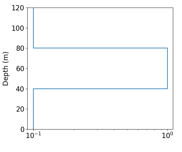
Here, we define the layer thicknesses and electrical conductivities for our 1D simulation. If we have N layers, we define N electrical conductivity values and N-1 layer thicknesses. The lowest layer is assumed to extend to infinity. If the Earth is a halfspace, the thicknesses can be defined by an empty array, and the physical property values by an array of length 1.
In this case, we have a more conductive layer within a background halfspace. This can be defined as a 3 layered Earth model.
# Physical properties
background_conductivity = 1e-1
layer_conductivity = 1e0

# Layer thicknesses
thicknesses = np.array([40.0, 40.0])
n_layer = len(thicknesses) + 1

# physical property models
model = background_conductivity * np.ones(n_layer)
model[1] = layer_conductivity

# Define a mapping for conductivities
model_mapping = maps.IdentityMap(nP=n_layer)

# Plot conductivity model
thicknesses_for_plotting = np.r_[thicknesses, 40.0]

fig = plt.figure(figsize=(6, 5))
ax = fig.add_axes([0.15, 0.15, 0.8, 0.8])
plot_1d_layer_model(thicknesses_for_plotting, model, ax=ax, show_layers=False)
plt.gca().invert_yaxis()

Define the Forward Simulation, Predict Data and Plot#
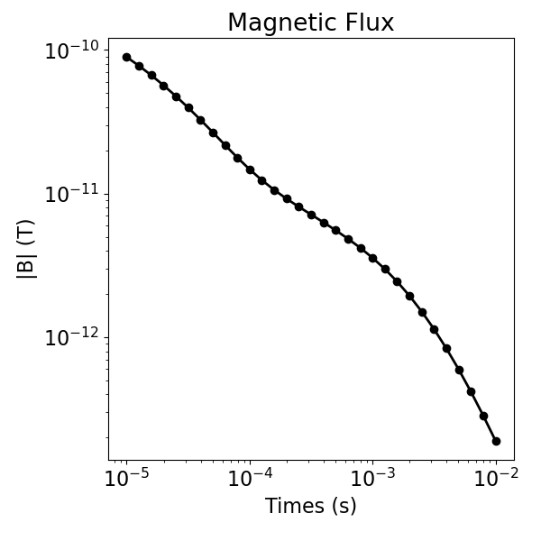
Here we define the simulation and predict the 1D TDEM sounding data. The simulation requires the user define the survey, the layer thicknesses and a mapping from the model to the conductivities of the layers.
When using the SimPEG.electromagnetics.time_domain_1d module, predicted data are organized by source, then by receiver, then by time channel.
# Define the simulation
simulation = tdem.Simulation1DLayered(
    survey=survey,
    thicknesses=thicknesses,
    sigmaMap=model_mapping,
)

# Predict data for a given model
dpred = simulation.dpred(model)

# Plot sounding
fig = plt.figure(figsize=(6, 6))
ax = fig.add_axes([0.2, 0.15, 0.75, 0.78])
ax.loglog(times, dpred, "k-o", lw=2)
ax.set_xlabel("Times (s)")
ax.set_ylabel("|B| (T)")
ax.set_title("Magnetic Flux")

Text(0.5, 1.0, 'Magnetic Flux')
Write Output (Optional)#
if write_output:
    dir_path = os.path.dirname(__file__).split(os.path.sep)
    dir_path.extend(["outputs"])
    dir_path = os.path.sep.join(dir_path) + os.path.sep

    if not os.path.exists(dir_path):
        os.mkdir(dir_path)

    np.random.seed(347)
    noise = 0.05 * np.abs(dpred) * np.random.rand(len(dpred))
    dpred += noise
    fname = dir_path + "em1dtm_data.txt"
    np.savetxt(fname, np.c_[times, dpred], fmt="%.4e", header="TIME BZ")
Total running time of the script: ( 0 minutes 4.088 seconds)
Estimated memory usage: 17 MB