simpeg.simulation.BaseTimeSimulation#
- class simpeg.simulation.BaseTimeSimulation(t0=0.0, time_steps=None, **kwargs)[source]#
Bases:
BaseSimulationBase class for time domain simulations.
The
BaseTimeSimulationdefines properties and methods that are required when the finite volume approach is used to solve time-dependent forward simulations. Presently, SimPEG discretizes in time using the backward Euler approach. And as such, the user must now define the step lengths for the forward simulation.- Parameters:
- t0
float,optional Initial time, in seconds, for the time-dependent forward simulation.
- time_steps(
n_steps, )numpy.ndarray,optional The time step lengths, in seconds, for the time domain simulation. This property can be also be set using a compact form; see Notes.
- t0
Attributes
A list of solver objects to clean when the model is updated
SimPEG
Counterobject to store iterations and run-times.HasModel.deleteTheseOnModelUpdate has been deprecated.
The inversion model.
Total number of time steps.
True if a model is necessary
Path to directory where sensitivity file is stored.
The survey for the simulation.
Initial time, in seconds, for the time-dependent forward simulation.
Time mesh for easy interpolation to observation times.
Time step lengths, in seconds, for the time domain simulation.
Evaluation times.
Verbose progress printout.
Methods
Jtvec(m, v[, f])Compute the Jacobian transpose times a vector for the model provided.
Jtvec_approx(m, v[, f])Approximation of the Jacobian transpose times a vector for the model provided.
Jvec(m, v[, f])Compute the Jacobian times a vector for the model provided.
Jvec_approx(m, v[, f])Approximation of the Jacobian times a vector for the model provided.
dpred([m, f])Predicted data for the model provided.
fields([m])Return the computed geophysical fields for the model provided.
make_synthetic_data(m[, relative_error, ...])Make synthetic data for the model and Gaussian noise provided.
residual(m, dobs[, f])The data residual.
Notes
There are two ways in which the user can set the
time_stepsproperty for the forward simulation. The most basic approach is to use a(n_steps, )numpy.ndarraythat explicitly defines the step lengths in order. I.e.:>>> sim.time_steps = np.r_[1e-6, 1e-6, 1e-6, 1e-5, 1e-5, 1e-4, 1e-4]
We can define also define the step lengths in compact for when the same step length is reused multiple times in succession. In this case, the
time_stepsproperty is set using alistoftuple. Eachtuplecontains the step length and number of times that step is repeated. The time stepping defined above can be set equivalently with:>>> sim.time_steps = [(1e-6, 3), (1e-5, 2), (1e-4, 2)]
When set, the
discretize.utils.unpack_widths()utility is used to convert thelistoftupleto its (n_steps, )numpy.ndarrayrepresentation.
Galleries and Tutorials using simpeg.simulation.BaseTimeSimulation#
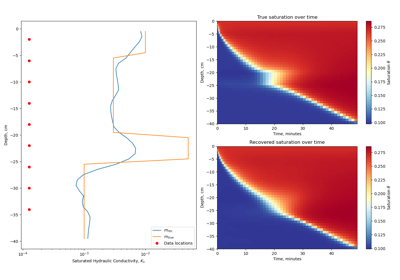
Time-domain CSEM for a resistive cube in a deep marine setting
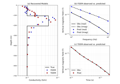
Heagy et al., 2017 1D RESOLVE and SkyTEM Bookpurnong Inversions
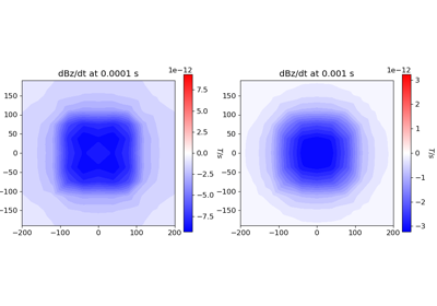
3D Forward Simulation for Transient Response on a Cylindrical Mesh

