simpeg.maps.SurjectVertical1D#
- class simpeg.maps.SurjectVertical1D(mesh, **kwargs)[source]#
Bases:
IdentityMapMap 1D layered Earth model to 2D or 3D tensor mesh.
Let \(m\) be a 1D model that defines the property values along the last dimension of a tensor mesh; i.e. the y-direction for 2D meshes and the z-direction for 3D meshes.
SurjectVertical1Dconstruct a surjective mapping from the 1D model to all voxel cells in the 2D or 3D tensor mesh provided.Mathematically, the mapping \(\mathbf{u}(\mathbf{m})\) can be represented by a projection matrix:
\[\mathbf{u}(\mathbf{m}) = \mathbf{Pm}\]- Parameters:
- mesh
discretize.TensorMesh A 2D or 3D tensor mesh
- mesh
Attributes
Determine whether or not this mapping is a linear operation.
The mesh used for the mapping
Number of parameters the mapping acts on.
Dimensions of the mapping operator
Methods
deriv(m[, v])Derivative of the mapping with respect to the model paramters.
dot(map1)Multiply two mappings to create a
simpeg.maps.ComboMap.inverse(D)The transform inverse is not implemented.
test([m, num, random_seed])Derivative test for the mapping.
Examples
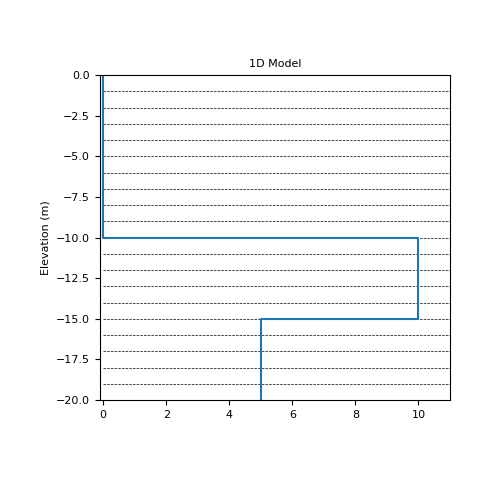
Here we define a 1D layered Earth model comprised of 3 layers on a 1D tensor mesh. We then use
SurjectVertical1Dto construct a mapping which projects the 1D model onto a 2D tensor mesh.>>> from simpeg.maps import SurjectVertical1D >>> from simpeg.utils import plot_1d_layer_model >>> from discretize import TensorMesh >>> import numpy as np >>> import matplotlib as mpl >>> import matplotlib.pyplot as plt
>>> dh = np.ones(20)
>>> mesh1D = TensorMesh([dh], 'C')
>>> mesh2D = TensorMesh([dh, dh], 'CC')
>>> m = np.zeros(mesh1D.nC)
>>> m[mesh1D.cell_centers < 0] = 10.
>>> m[mesh1D.cell_centers < -5] = 5.
>>> fig1 = plt.figure(figsize=(5,5))
>>> ax1 = fig1.add_subplot(111)
>>> plot_1d_layer_model(
>>>     mesh1D.h[0], np.flip(m), ax=ax1, z0=0,
>>>     scale='linear', show_layers=True, plot_elevation=True
>>> )
>>> ax1.set_xlim([-0.1, 11])
>>> ax1.set_title('1D Model')
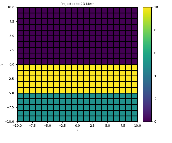
>>> mapping = SurjectVertical1D(mesh2D)
>>> u = mapping * m
>>> fig2 = plt.figure(figsize=(6, 5))
>>> ax2a = fig2.add_axes([0.1, 0.15, 0.7, 0.8])
>>> mesh2D.plot_image(u, ax=ax2a, grid=True)
>>> ax2a.set_title('Projected to 2D Mesh')
>>> ax2b = fig2.add_axes([0.83, 0.15, 0.05, 0.8])
>>> norm = mpl.colors.Normalize(vmin=np.min(m), vmax=np.max(m))
>>> cbar = mpl.colorbar.ColorbarBase(ax2b, norm=norm, orientation="vertical")

Galleries and Tutorials using simpeg.maps.SurjectVertical1D#
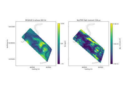
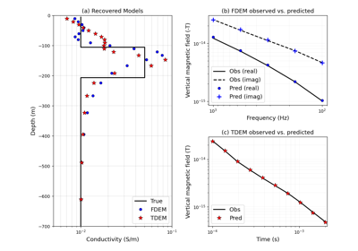
Heagy et al., 2017 1D RESOLVE and SkyTEM Bookpurnong Inversions
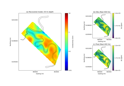
Heagy et al., 2017 1D RESOLVE Bookpurnong Inversion