Note
Click here to download the full example code
EM: TDEM: Permeable Target, Inductive Source#
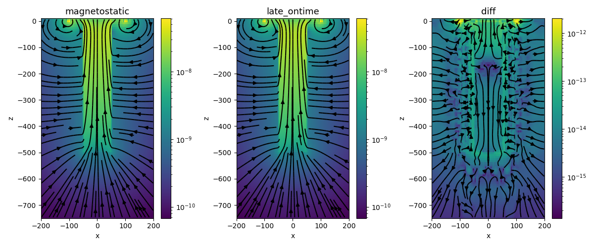
In this example, we demonstrate 2 approaches for simulating TDEM data when a permeable target is present in the simulation domain. In the first, we use a step-on waveform (QuarterSineRampOnWaveform) and look at the magnetic flux at a late on-time. In the second, we solve the magnetostatic problem to compute the initial magnetic flux so that a step-off waveform may be used.
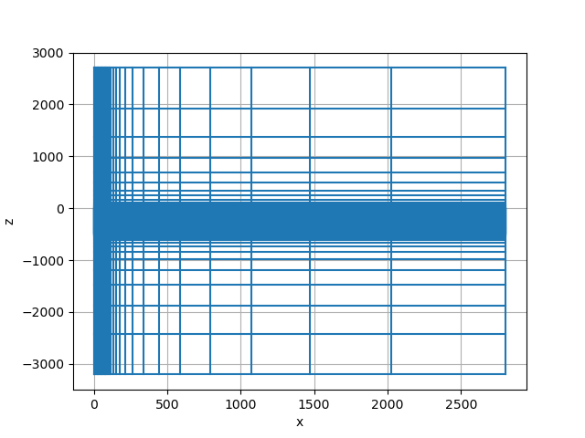
A cylindrically symmetric mesh is employed and a circular loop source is used
import discretize
import numpy as np
import matplotlib.pyplot as plt
from matplotlib.colors import LogNorm
from scipy.constants import mu_0

try:
    from pymatsolver import Pardiso as Solver
except ImportError:
    from SimPEG import SolverLU as Solver
import time

from SimPEG.electromagnetics import time_domain as TDEM
from SimPEG import utils, maps, Report
Model Parameters#
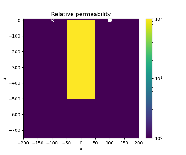
Here, we define our simulation parameters. The target has a relative permeability of 100 \(\mu_0\)
target_mur = 100  # permeability of the target
target_l = 500  # length of target
target_r = 50  # radius of the target

sigma_back = 1e-5  # conductivity of the background

radius_loop = 100  # radius of the transmitter loop
Mesh#
Next, we create a cylindrically symmteric tensor mesh
csx = 5.0  # core cell size in the x-direction
csz = 5.0  # core cell size in the z-direction
domainx = 100  # use a uniform cell size out to a radius of 100m

# padding parameters
npadx, npadz = 15, 15  # number of padding cells
pfx = 1.4  # expansion factor for the padding to infinity in the x-direction
pfz = 1.4  # expansion factor for the padding to infinity in the z-direction

ncz = int(target_l / csz)  # number of z cells in the core region

# create the cyl mesh
mesh = discretize.CylindricalMesh(
    [
        [(csx, int(domainx / csx)), (csx, npadx, pfx)],
        1,
        [(csz, npadz, -pfz), (csz, ncz), (csz, npadz, pfz)],
    ]
)

# put the origin at the top of the target
mesh.x0 = [0, 0, -mesh.h[2][: npadz + ncz].sum()]

# plot the mesh
mesh.plot_grid()
<AxesSubplot:xlabel='x', ylabel='z'>
Assign physical properties on the mesh
mur_model = np.ones(mesh.nC)

# find the indices of the target
x_inds = mesh.gridCC[:, 0] < target_r
z_inds = (mesh.gridCC[:, 2] <= 0) & (mesh.gridCC[:, 2] >= -target_l)

mur_model[x_inds & z_inds] = target_mur
mu_model = mu_0 * mur_model

sigma = np.ones(mesh.nC) * sigma_back
Plot the models
xlim = np.r_[-200, 200]  # x-limits in meters
zlim = np.r_[-1.5 * target_l, 10.0]  # z-limits in meters. (z-positive up)

fig, ax = plt.subplots(1, 1, figsize=(6, 5))

# plot the permeability
plt.colorbar(
    mesh.plot_image(
        mur_model,
        ax=ax,
        pcolor_opts={"norm": LogNorm()},  # plot on a log-scale
        mirror=True,
    )[0],
    ax=ax,
)
ax.plot(np.r_[radius_loop], np.r_[0.0], "wo", markersize=8)
ax.plot(np.r_[-radius_loop], np.r_[0.0], "wx", markersize=8)

ax.set_title("Relative permeability", fontsize=13)
ax.set_xlim(xlim)
ax.set_ylim(zlim)
(-750.0, 10.0)
Waveform for the Long On-Time Simulation#
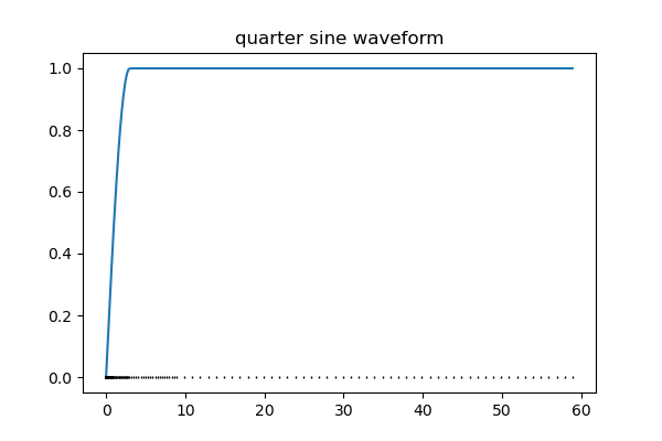
Here, we define our time-steps for the simulation where we will use a waveform with a long on-time to reach a steady-state magnetic field and define a quarter-sine ramp-on waveform as our transmitter waveform
ramp = [
    (1e-5, 20),
    (1e-4, 20),
    (3e-4, 20),
    (1e-3, 20),
    (3e-3, 20),
    (1e-2, 20),
    (3e-2, 20),
    (1e-1, 20),
    (3e-1, 20),
    (1, 50),
]
time_mesh = discretize.TensorMesh([ramp])

# define an off time past when we will simulate to keep the transmitter on
off_time = 100
quarter_sine = TDEM.Src.QuarterSineRampOnWaveform(
    ramp_on=np.r_[0.0, 3], ramp_off=off_time - np.r_[1.0, 0]
)

# evaluate the waveform at each time in the simulation
quarter_sine_plt = [quarter_sine.eval(t) for t in time_mesh.gridN]

fig, ax = plt.subplots(1, 1, figsize=(6, 4))
ax.plot(time_mesh.gridN, quarter_sine_plt)
ax.plot(time_mesh.gridN, np.zeros(time_mesh.nN), "k|", markersize=2)
ax.set_title("quarter sine waveform")
Text(0.5, 1.0, 'quarter sine waveform')
Sources for the 2 simulations#
We use two sources, one for the magnetostatic simulation and one for the ramp on simulation.
# For the magnetostatic simulation. The default waveform is a step-off
src_magnetostatic = TDEM.Src.CircularLoop(
    [],
    location=np.r_[0.0, 0.0, 0.0],
    orientation="z",
    radius=100,
)

# For the long on-time simulation. We use the ramp-on waveform
src_ramp_on = TDEM.Src.CircularLoop(
    [],
    location=np.r_[0.0, 0.0, 0.0],
    orientation="z",
    radius=100,
    waveform=quarter_sine,
)

src_list_magnetostatic = [src_magnetostatic]
src_list_ramp_on = [src_ramp_on]
Create the simulations#
To simulate magnetic flux data, we use the b-formulation of Maxwell’s equations
survey_magnetostatic = TDEM.Survey(source_list=src_list_magnetostatic)
survey_ramp_on = TDEM.Survey(src_list_ramp_on)

prob_magnetostatic = TDEM.Simulation3DMagneticFluxDensity(
    mesh=mesh,
    survey=survey_magnetostatic,
    sigmaMap=maps.IdentityMap(mesh),
    time_steps=ramp,
    solver=Solver,
)
prob_ramp_on = TDEM.Simulation3DMagneticFluxDensity(
    mesh=mesh,
    survey=survey_ramp_on,
    sigmaMap=maps.IdentityMap(mesh),
    time_steps=ramp,
    solver=Solver,
)
Run the long on-time simulation#
--- Running Long On-Time Simulation ---
 ... done. Elapsed time 1.3936305046081543
Compute Magnetostatic Fields from the step-off source#
prob_magnetostatic.mu = mu_model
prob_magnetostatic.model = sigma
b_magnetostatic = src_magnetostatic.bInitial(prob_magnetostatic)
Plot the results#
def plotBFieldResults(
    ax=None,
    clim_min=None,
    clim_max=None,
    max_depth=1.5 * target_l,
    max_r=100,
    top=10.0,
    view="magnetostatic",
):
    if ax is None:
        plt.subplots(1, 1, figsize=(6, 7))

    assert view.lower() in ["magnetostatic", "late_ontime", "diff"]

    xlim = max_r * np.r_[-1, 1]  # x-limits in meters
    zlim = np.r_[-max_depth, top]  # z-limits in meters. (z-positive up)

    clim = None

    if clim_max is not None and clim_max != 0.0:
        clim = clim_max * np.r_[-1, 1]

        if clim_min is not None and clim_min != 0.0:
            clim[0] = clim_min

    if view == "magnetostatic":
        plotme = b_magnetostatic
    elif view == "late_ontime":
        plotme = b_ramp_on
    elif view == "diff":
        plotme = b_magnetostatic - b_ramp_on

    cb = plt.colorbar(
        mesh.plot_image(
            plotme,
            view="vec",
            v_type="F",
            ax=ax,
            range_x=xlim,
            range_y=zlim,
            sample_grid=np.r_[np.diff(xlim) / 100.0, np.diff(zlim) / 100.0],
            mirror=True,
            pcolor_opts={"norm": LogNorm()},
        )[0],
        ax=ax,
    )
    ax.set_title("{}".format(view), fontsize=13)
    ax.set_xlim(xlim)
    ax.set_ylim(zlim)
    cb.update_ticks()

    return ax


fig, ax = plt.subplots(1, 3, figsize=(12, 5))

for a, v in zip(ax, ["magnetostatic", "late_ontime", "diff"]):
    a = plotBFieldResults(ax=a, clim_min=1e-15, clim_max=1e-7, view=v, max_r=200)
plt.tight_layout()
Print the version of SimPEG and dependencies#
plt.show()

Report()
Total running time of the script: ( 0 minutes 8.803 seconds)
Estimated memory usage: 18 MB