FLOW: Richards: 1D: Celia1990

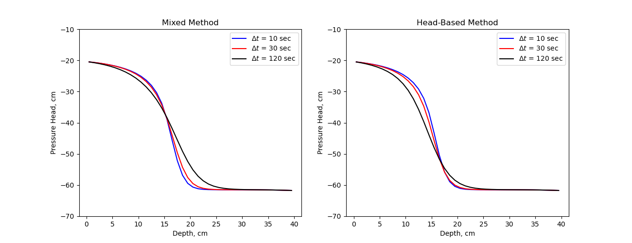
There are two different forms of Richards equation that differ on how they deal with the non-linearity in the time-stepping term.

The most fundamental form, referred to as the ‘mixed’-form of Richards Equation Celia1990

\[\frac{\partial \theta(\psi)}{\partial t} - \nabla \cdot k(\psi) \nabla \psi - \frac{\partial k(\psi)}{\partial z} = 0 \quad \psi \in \Omega\]

where \(\theta\) is water content, and \(\psi\) is pressure head. This formulation of Richards equation is called the ‘mixed’-form because the equation is parameterized in \(\psi\) but the time-stepping is in terms of \(\theta\).

As noted in Celia1990 the ‘head’-based form of Richards equation can be written in the continuous form as:

\[\frac{\partial \theta}{\partial \psi} \frac{\partial \psi}{\partial t} - \nabla \cdot k(\psi) \nabla \psi - \frac{\partial k(\psi)}{\partial z} = 0 \quad \psi \in \Omega\]

However, it can be shown that this does not conserve mass in the discrete formulation.

Here we reproduce the results from Celia1990 demonstrating the head-based formulation and the mixed-formulation.

/usr/share/miniconda/envs/test/lib/python3.7/site-packages/discretize/operators/differential_operators.py:1795: UserWarning:

cell_gradient_BC is deprecated and is not longer used. See cell_gradient

import matplotlib.pyplot as plt
import numpy as np

import discretize
from SimPEG import maps
from SimPEG.flow import richards


def run(plotIt=True):

    M = discretize.TensorMesh([np.ones(40)])
    M.set_cell_gradient_BC("dirichlet")
    params = richards.empirical.HaverkampParams().celia1990
    k_fun, theta_fun = richards.empirical.haverkamp(M, **params)
    k_fun.KsMap = maps.IdentityMap(nP=M.nC)

    bc = np.array([-61.5, -20.7])
    h = np.zeros(M.nC) + bc[0]

    def getFields(timeStep, method):
        timeSteps = np.ones(int(360 / timeStep)) * timeStep
        prob = richards.SimulationNDCellCentered(
            M,
            hydraulic_conductivity=k_fun,
            water_retention=theta_fun,
            boundary_conditions=bc,
            initial_conditions=h,
            do_newton=False,
            method=method,
        )
        prob.time_steps = timeSteps
        return prob.fields(params["Ks"] * np.ones(M.nC))

    Hs_M010 = getFields(10, "mixed")
    Hs_M030 = getFields(30, "mixed")
    Hs_M120 = getFields(120, "mixed")
    Hs_H010 = getFields(10, "head")
    Hs_H030 = getFields(30, "head")
    Hs_H120 = getFields(120, "head")

    if not plotIt:
        return
    plt.figure(figsize=(13, 5))
    plt.subplot(121)
    plt.plot(40 - M.gridCC, Hs_M010[-1], "b-")
    plt.plot(40 - M.gridCC, Hs_M030[-1], "r-")
    plt.plot(40 - M.gridCC, Hs_M120[-1], "k-")
    plt.ylim([-70, -10])
    plt.title("Mixed Method")
    plt.xlabel("Depth, cm")
    plt.ylabel("Pressure Head, cm")
    plt.legend(("$\Delta t$ = 10 sec", "$\Delta t$ = 30 sec", "$\Delta t$ = 120 sec"))
    plt.subplot(122)
    plt.plot(40 - M.gridCC, Hs_H010[-1], "b-")
    plt.plot(40 - M.gridCC, Hs_H030[-1], "r-")
    plt.plot(40 - M.gridCC, Hs_H120[-1], "k-")
    plt.ylim([-70, -10])
    plt.title("Head-Based Method")
    plt.xlabel("Depth, cm")
    plt.ylabel("Pressure Head, cm")
    plt.legend(("$\Delta t$ = 10 sec", "$\Delta t$ = 30 sec", "$\Delta t$ = 120 sec"))


if __name__ == "__main__":
    run()
    plt.show()

Estimated memory usage: 18 MB