Note
Click here to download the full example code
EM: Schenkel and Morrison Casing Model#
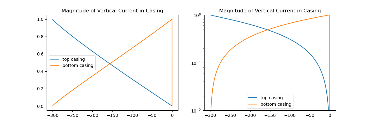
Here we create and run a FDEM forward simulation to calculate the vertical current inside a steel-cased. The model is based on the Schenkel and Morrison Casing Model, and the results are used in a 2016 SEG abstract by Yang et al.
Schenkel, C.J., and H.F. Morrison, 1990, Effects of well casing on
potential field measurements using downhole current sources:
Geophysical prospecting, 38, 663-686.
The model consists of:
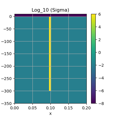
Air: Conductivity 1e-8 S/m, above z = 0
Background: conductivity 1e-2 S/m, below z = 0
- Casing: conductivity 1e6 S/m
300m long
radius of 0.1m
thickness of 6e-3m
Inside the casing, we take the same conductivity as the background.
We are using an EM code to simulate DC, so we use frequency low enough that the skin depth inside the casing is longer than the casing length (f = 1e-6 Hz). The plot produced is of the current inside the casing.
These results are shown in the SEG abstract by Yang et al., 2016: 3D DC resistivity modeling of steel casing for reservoir monitoring using equivalent resistor network. The solver used to produce these results and achieve the CPU time of ~30s is Mumps, which was installed using pymatsolver
This example is on figshare: https://dx.doi.org/10.6084/m9.figshare.3126961.v1
If you would use this example for a code comparison, or build upon it, a citation would be much appreciated!
Skin Depth:  [5000000.0]
/home/vsts/work/1/s/examples/20-published/plot_schenkel_morrison_casing.py:112: DeprecationWarning:

`np.int` is a deprecated alias for the builtin `int`. To silence this warning, use `int` by itself. Doing this will not modify any behavior and is safe. When replacing `np.int`, you may wish to use e.g. `np.int64` or `np.int32` to specify the precision. If you wish to review your current use, check the release note link for additional information.
Deprecated in NumPy 1.20; for more details and guidance: https://numpy.org/devdocs/release/1.20.0-notes.html#deprecations

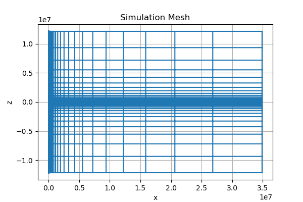
Mesh Extent xmax: 30844847.844048,: zmin: -10732642.852316, zmax: 10732343.352316
Number of cells 878878
Time to solve 2 sources 9.844954013824463
from __future__ import print_function
import matplotlib.pylab as plt
import numpy as np
import discretize
from SimPEG import maps, utils
from SimPEG.electromagnetics import frequency_domain as FDEM
import time

try:
    from pymatsolver import Pardiso as Solver
except Exception:
    from SimPEG import SolverLU as Solver


def run(plotIt=True):

    # ------------------ MODEL ------------------
    sigmaair = 1e-8  # air
    sigmaback = 1e-2  # background
    sigmacasing = 1e6  # casing
    sigmainside = sigmaback  # inside the casing

    casing_t = 0.006  # 1cm thickness
    casing_l = 300  # length of the casing

    casing_r = 0.1
    casing_a = casing_r - casing_t / 2.0  # inner radius
    casing_b = casing_r + casing_t / 2.0  # outer radius
    casing_z = np.r_[-casing_l, 0.0]

    # ------------------ SURVEY PARAMETERS ------------------
    freqs = np.r_[1e-6]  # [1e-1, 1, 5] # frequencies
    dsz = -300  # down-hole z source location
    src_loc = np.r_[0.0, 0.0, dsz]
    inf_loc = np.r_[0.0, 0.0, 1e4]

    print("Skin Depth: ", [(500.0 / np.sqrt(sigmaback * _)) for _ in freqs])

    # ------------------ MESH ------------------
    # fine cells near well bore
    csx1, csx2 = 2e-3, 60.0
    pfx1, pfx2 = 1.3, 1.3
    ncx1 = np.ceil(casing_b / csx1 + 2)

    # pad nicely to second cell size
    npadx1 = np.floor(np.log(csx2 / csx1) / np.log(pfx1))
    hx1a = utils.unpack_widths([(csx1, ncx1)])
    hx1b = utils.unpack_widths([(csx1, npadx1, pfx1)])
    dx1 = sum(hx1a) + sum(hx1b)
    dx1 = np.floor(dx1 / csx2)
    hx1b *= (dx1 * csx2 - sum(hx1a)) / sum(hx1b)

    # second chunk of mesh
    dx2 = 300.0  # uniform mesh out to here
    ncx2 = np.ceil((dx2 - dx1) / csx2)
    npadx2 = 45
    hx2a = utils.unpack_widths([(csx2, ncx2)])
    hx2b = utils.unpack_widths([(csx2, npadx2, pfx2)])
    hx = np.hstack([hx1a, hx1b, hx2a, hx2b])

    # z-direction
    csz = 0.05
    nza = 10
    # cell size, number of core cells, number of padding cells in the
    # x-direction
    ncz, npadzu, npadzd = np.int(np.ceil(np.diff(casing_z)[0] / csz)) + 10, 68, 68
    # vector of cell widths in the z-direction
    hz = utils.unpack_widths([(csz, npadzd, -1.3), (csz, ncz), (csz, npadzu, 1.3)])

    # Mesh
    mesh = discretize.CylindricalMesh(
        [hx, 1.0, hz], [0.0, 0.0, -np.sum(hz[: npadzu + ncz - nza])]
    )

    print(
        "Mesh Extent xmax: {0:f},: zmin: {1:f}, zmax: {2:f}".format(
            mesh.cell_centers_x.max(),
            mesh.cell_centers_z.min(),
            mesh.cell_centers_z.max(),
        )
    )
    print("Number of cells", mesh.nC)

    if plotIt is True:
        fig, ax = plt.subplots(1, 1, figsize=(6, 4))
        ax.set_title("Simulation Mesh")
        mesh.plot_grid(ax=ax)

    # Put the model on the mesh
    sigWholespace = sigmaback * np.ones((mesh.nC))

    sigBack = sigWholespace.copy()
    sigBack[mesh.gridCC[:, 2] > 0.0] = sigmaair

    sigCasing = sigBack.copy()
    iCasingZ = (mesh.gridCC[:, 2] <= casing_z[1]) & (mesh.gridCC[:, 2] >= casing_z[0])
    iCasingX = (mesh.gridCC[:, 0] >= casing_a) & (mesh.gridCC[:, 0] <= casing_b)
    iCasing = iCasingX & iCasingZ
    sigCasing[iCasing] = sigmacasing

    if plotIt is True:
        # plotting parameters
        xlim = np.r_[0.0, 0.2]
        zlim = np.r_[-350.0, 10.0]
        clim_sig = np.r_[-8, 6]

        # plot models
        fig, ax = plt.subplots(1, 1, figsize=(4, 4))

        im = mesh.plot_image(np.log10(sigCasing), ax=ax)[0]
        im.set_clim(clim_sig)
        plt.colorbar(im, ax=ax)
        ax.grid(which="both")
        ax.set_title("Log_10 (Sigma)")
        ax.set_xlim(xlim)
        ax.set_ylim(zlim)

    # -------------- Sources --------------------
    # Define Custom Current Sources

    # surface source
    sg_x = np.zeros(mesh.vnF[0], dtype=complex)
    sg_y = np.zeros(mesh.vnF[1], dtype=complex)
    sg_z = np.zeros(mesh.vnF[2], dtype=complex)

    nza = 2  # put the wire two cells above the surface

    # vertically directed wire
    # hook it up to casing at the surface
    sgv_indx = (mesh.gridFz[:, 0] > casing_a) & (mesh.gridFz[:, 0] < casing_a + csx1)
    sgv_indz = (mesh.gridFz[:, 2] <= +csz * nza) & (mesh.gridFz[:, 2] >= -csz * 2)
    sgv_ind = sgv_indx & sgv_indz
    sg_z[sgv_ind] = -1.0

    # horizontally directed wire
    sgh_indx = (mesh.gridFx[:, 0] > casing_a) & (mesh.gridFx[:, 0] <= inf_loc[2])
    sgh_indz = (mesh.gridFx[:, 2] > csz * (nza - 0.5)) & (
        mesh.gridFx[:, 2] < csz * (nza + 0.5)
    )
    sgh_ind = sgh_indx & sgh_indz
    sg_x[sgh_ind] = -1.0

    # hook it up to casing at the surface
    sgv2_indx = (mesh.gridFz[:, 0] >= mesh.gridFx[sgh_ind, 0].max()) & (
        mesh.gridFz[:, 0] <= inf_loc[2] * 1.2
    )
    sgv2_indz = (mesh.gridFz[:, 2] <= +csz * nza) & (mesh.gridFz[:, 2] >= -csz * 2)
    sgv2_ind = sgv2_indx & sgv2_indz
    sg_z[sgv2_ind] = 1.0

    # assemble the source
    sg = np.hstack([sg_x, sg_y, sg_z])
    sg_p = [FDEM.Src.RawVec_e([], _, sg / mesh.face_areas) for _ in freqs]

    # downhole source
    dg_x = np.zeros(mesh.vnF[0], dtype=complex)
    dg_y = np.zeros(mesh.vnF[1], dtype=complex)
    dg_z = np.zeros(mesh.vnF[2], dtype=complex)

    # vertically directed wire
    dgv_indx = mesh.gridFz[:, 0] < csx1  # go through the center of the well
    dgv_indz = (mesh.gridFz[:, 2] <= +csz * nza) & (mesh.gridFz[:, 2] > dsz + csz / 2.0)
    dgv_ind = dgv_indx & dgv_indz
    dg_z[dgv_ind] = -1.0

    # couple to the casing downhole
    dgh_indx = mesh.gridFx[:, 0] < casing_a + csx1
    dgh_indz = (mesh.gridFx[:, 2] < dsz + csz) & (mesh.gridFx[:, 2] >= dsz)
    dgh_ind = dgh_indx & dgh_indz
    dg_x[dgh_ind] = 1.0

    # horizontal part at surface
    dgh2_indx = mesh.gridFx[:, 0] <= inf_loc[2] * 1.2
    dgh2_indz = sgh_indz.copy()
    dgh2_ind = dgh2_indx & dgh2_indz
    dg_x[dgh2_ind] = -1.0

    # vertical part at surface
    dgv2_ind = sgv2_ind.copy()
    dg_z[dgv2_ind] = 1.0

    # assemble the source
    dg = np.hstack([dg_x, dg_y, dg_z])
    dg_p = [FDEM.Src.RawVec_e([], _, dg / mesh.face_areas) for _ in freqs]

    # ------------ Problem and Survey ---------------
    survey = FDEM.Survey(sg_p + dg_p)
    problem = FDEM.Simulation3DMagneticField(
        mesh, survey=survey, sigmaMap=maps.IdentityMap(mesh), solver=Solver
    )

    # ------------- Solve ---------------------------
    t0 = time.time()
    fieldsCasing = problem.fields(sigCasing)
    print("Time to solve 2 sources", time.time() - t0)

    # Plot current

    # current density
    jn0 = fieldsCasing[dg_p, "j"]
    jn1 = fieldsCasing[sg_p, "j"]

    # current
    in0 = [mesh.face_areas * fieldsCasing[dg_p, "j"][:, i] for i in range(len(freqs))]
    in1 = [mesh.face_areas * fieldsCasing[sg_p, "j"][:, i] for i in range(len(freqs))]

    in0 = np.vstack(in0).T
    in1 = np.vstack(in1).T

    # integrate to get z-current inside casing
    inds_inx = (mesh.gridFz[:, 0] >= casing_a) & (mesh.gridFz[:, 0] <= casing_b)
    inds_inz = (mesh.gridFz[:, 2] >= dsz) & (mesh.gridFz[:, 2] <= 0)
    inds_fz = inds_inx & inds_inz

    indsx = [False] * mesh.nFx
    inds = list(indsx) + list(inds_fz)

    in0_in = in0[np.r_[inds]]
    in1_in = in1[np.r_[inds]]
    z_in = mesh.gridFz[inds_fz, 2]

    in0_in = in0_in.reshape([in0_in.shape[0] // 3, 3])
    in1_in = in1_in.reshape([in1_in.shape[0] // 3, 3])
    z_in = z_in.reshape([z_in.shape[0] // 3, 3])

    I0 = in0_in.sum(1).real
    I1 = in1_in.sum(1).real
    z_in = z_in[:, 0]

    if plotIt is True:
        fig, ax = plt.subplots(1, 2, figsize=(12, 4))

        ax[0].plot(z_in, np.absolute(I0), z_in, np.absolute(I1))
        ax[0].legend(["top casing", "bottom casing"], loc="best")
        ax[0].set_title("Magnitude of Vertical Current in Casing")

        ax[1].semilogy(z_in, np.absolute(I0), z_in, np.absolute(I1))
        ax[1].legend(["top casing", "bottom casing"], loc="best")
        ax[1].set_title("Magnitude of Vertical Current in Casing")
        ax[1].set_ylim([1e-2, 1.0])


if __name__ == "__main__":
    run()
    plt.show()
Total running time of the script: ( 0 minutes 12.040 seconds)
Estimated memory usage: 1895 MB


