Note
Click here to download the full example code
FLOW: Richards: 1D: Forward Simulation#
The example shows simulation of Richards equation in 1D with a heterogeneous hydraulic conductivity function.
The haverkamp model is used with the same parameters as Celia1990 the boundary and initial conditions are also the same. The simulation domain is 40cm deep and is run for an hour with an exponentially increasing time step that has a maximum of one minute. The general setup of the experiment is an infiltration front that advances downward through the model over time.
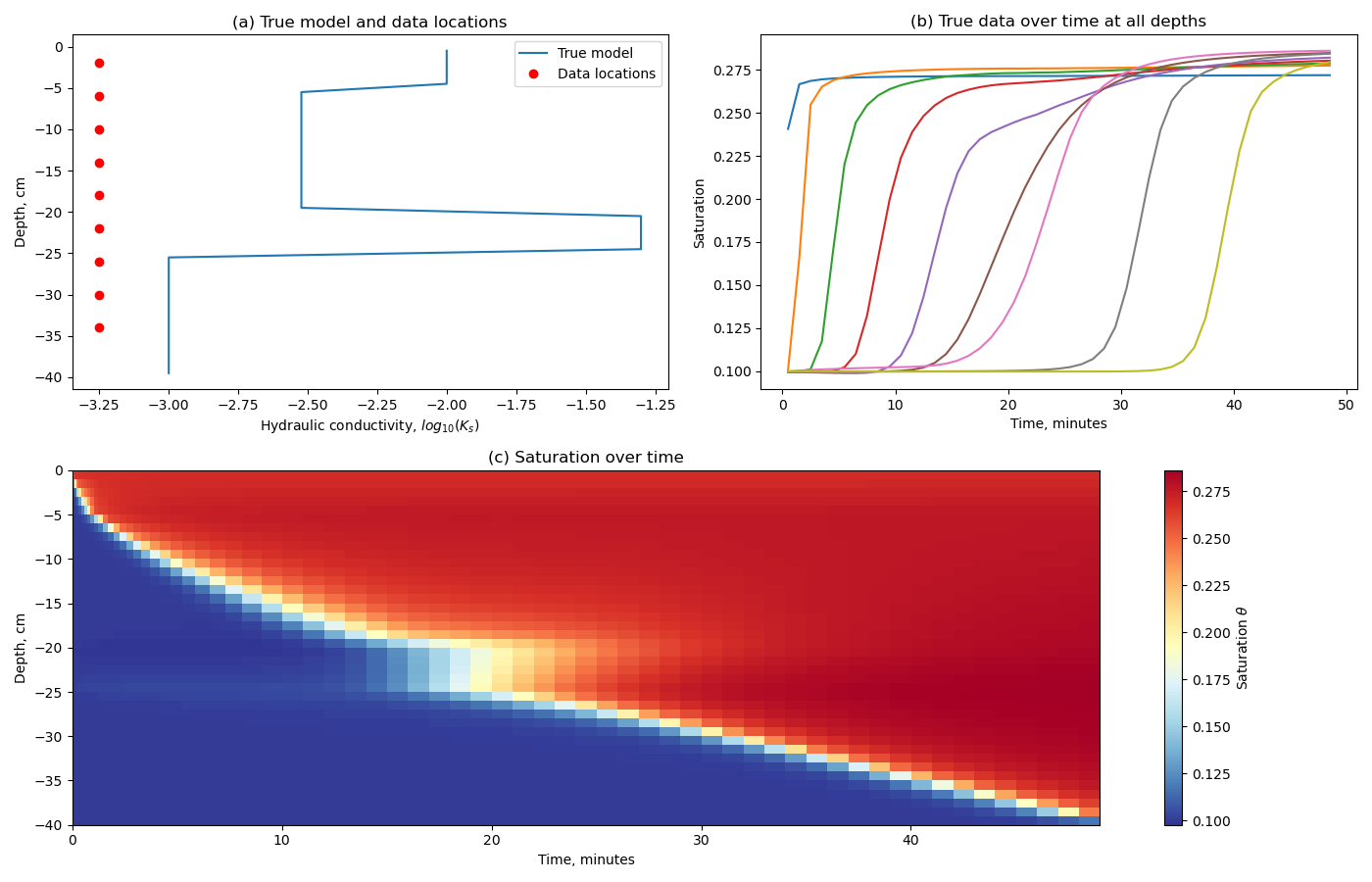
Figure (a) shows the heterogeneous saturated hydraulic conductivity parameter and the location of the data collection, which happens every minute from 30 seconds into the simulation. Note that the simulation mesh and the data locations are not aligned, and linear interpolation is used to collect the data. The points are sampled in pressure head and then transformed to saturation using the haverkamp model for the water retention curve.
Figure (b) shows the data collected from the simulation. No noise is added to the data at this time. The various data locations register the infiltration event through increasing saturation as the front moves past the receiver. Notice that the slope of the curves are not equal as the hydraulic conductivity function is heterogeneous.
Figure (c) shows the saturation field over the entire experiment. Here you can see that the timestep is not constant over time (5 seconds at the start of the simulation, 60 seconds at the end). You can also see the effect of the highly conductive layer in the model between 20 and 25 cm depth. The water drains straight through the conductive unit and piles up on the other side - advancing the fluid front faster than the other layers.
Rowan Cockett - 21/12/2016

/usr/share/miniconda/envs/test/lib/python3.7/site-packages/discretize/operators/differential_operators.py:1795: UserWarning:

cell_gradient_BC is deprecated and is not longer used. See cell_gradient
import matplotlib
import matplotlib.pyplot as plt
import numpy as np

import discretize
from SimPEG import maps
from SimPEG.flow import richards


def run(plotIt=True):

    M = discretize.TensorMesh([np.ones(40)], x0="N")
    M.set_cell_gradient_BC("dirichlet")
    # We will use the haverkamp empirical model with parameters from Celia1990
    k_fun, theta_fun = richards.empirical.haverkamp(
        M,
        A=1.1750e06,
        gamma=4.74,
        alpha=1.6110e06,
        theta_s=0.287,
        theta_r=0.075,
        beta=3.96,
    )

    # Here we are making saturated hydraulic conductivity
    # an exponential mapping to the model (defined below)
    k_fun.KsMap = maps.ExpMap(nP=M.nC)

    # Setup the boundary and initial conditions
    bc = np.array([-61.5, -20.7])
    h = np.zeros(M.nC) + bc[0]
    prob = richards.SimulationNDCellCentered(
        M,
        hydraulic_conductivity=k_fun,
        water_retention=theta_fun,
        boundary_conditions=bc,
        initial_conditions=h,
        do_newton=False,
        method="mixed",
        debug=False,
    )
    prob.time_steps = [(5, 25, 1.1), (60, 40)]

    # Create the survey
    locs = -np.arange(2, 38, 4.0).reshape(-1, 1)
    times = np.arange(30, prob.time_mesh.cell_centers_x[-1], 60)
    rxSat = richards.receivers.Saturation(locs, times)
    survey = richards.Survey([rxSat])
    prob.survey = survey

    # Create a simple model for Ks
    Ks = 1e-3
    mtrue = np.ones(M.nC) * np.log(Ks)
    mtrue[15:20] = np.log(5e-2)
    mtrue[20:35] = np.log(3e-3)
    mtrue[35:40] = np.log(1e-2)

    # Create some synthetic data and fields
    Hs = prob.fields(mtrue)
    data = prob.make_synthetic_data(mtrue, f=Hs)

    if plotIt:
        plt.figure(figsize=(14, 9))

        plt.subplot(221)
        plt.plot(np.log10(np.exp(mtrue)), M.gridCC)
        plt.title("(a) True model and data locations")
        plt.ylabel("Depth, cm")
        plt.xlabel("Hydraulic conductivity, $log_{10}(K_s)$")
        plt.plot([-3.25] * len(locs), locs, "ro")
        plt.legend(("True model", "Data locations"))

        plt.subplot(222)
        plt.plot(times / 60, data.dobs.reshape((-1, len(locs))))
        plt.title("(b) True data over time at all depths")
        plt.xlabel("Time, minutes")
        plt.ylabel("Saturation")

        ax = plt.subplot(212)
        mesh2d = discretize.TensorMesh([prob.time_mesh.h[0] / 60, prob.mesh.h[0]], "0N")
        sats = [theta_fun(_) for _ in Hs]
        clr = mesh2d.plot_image(np.c_[sats][1:, :], ax=ax)
        cmap0 = matplotlib.cm.RdYlBu_r
        clr[0].set_cmap(cmap0)
        c = plt.colorbar(clr[0])
        c.set_label("Saturation $\\theta$")
        plt.xlabel("Time, minutes")
        plt.ylabel("Depth, cm")
        plt.title("(c) Saturation over time")

        plt.tight_layout()


if __name__ == "__main__":
    run()
    plt.show()
Total running time of the script: ( 0 minutes 2.665 seconds)
Estimated memory usage: 18 MB