simpeg.electromagnetics.time_domain.Simulation3DElectricField

class simpeg.electromagnetics.time_domain.Simulation3DElectricField(mesh, survey=None, dt_threshold=1e-08, **kwargs)

Bases: BaseTDEMSimulation

3D TDEM simulation in terms of the electric field.

This simulation solves for the electric field at each time-step. In this formulation, the electric fields are defined on mesh edges and the magnetic flux density is defined on mesh faces; i.e. it is an EB formulation. See the Notes section for a comprehensive description of the formulation.

Parameters:

meshdiscretize.base.BaseMesh

The mesh.

surveytime_domain.survey.Survey

The time-domain EM survey.

dt_thresholdfloat

Threshold used when determining the unique time-step lengths.

Notes

Here, we start with the quasi-static approximation for Maxwell’s equations by neglecting electric displacement:

\[\begin{split}&\nabla \times \vec{e} + \frac{\partial \vec{b}}{\partial t} = - \frac{\partial \vec{s}_m}{\partial t} \\ &\nabla \times \vec{h} - \vec{j} = \vec{s}_e\end{split}\]

where \(\vec{s}_e\) is an electric source term that defines a source current density, and \(\vec{s}_m\) magnetic source term that defines a source magnetic flux density. We define the constitutive relations for the electrical conductivity \(\sigma\) and magnetic permeability \(\mu\) as:

\[\begin{split}\vec{j} &= \sigma \vec{e} \\ \vec{h} &= \mu^{-1} \vec{b}\end{split}\]

We then take the inner products of all previous expressions with a vector test function \(\vec{u}\). Through vector calculus identities and the divergence theorem, we obtain:

\[\begin{split}& \int_\Omega \vec{u} \cdot (\nabla \times \vec{e}) \, dv + \int_\Omega \vec{u} \cdot \frac{\partial \vec{b}}{\partial t} \, dv = - \int_\Omega \vec{u} \cdot \frac{\partial \vec{s}_m}{\partial t} \, dv \\ & \int_\Omega (\nabla \times \vec{u}) \cdot \vec{h} \, dv - \oint_{\partial \Omega} \vec{u} \cdot (\vec{h} \times \hat{n}) \, da - \int_\Omega \vec{u} \cdot \vec{j} \, dv = \int_\Omega \vec{u} \cdot \vec{s}_e \, dv \\ & \int_\Omega \vec{u} \cdot \vec{j} \, dv = \int_\Omega \vec{u} \cdot \sigma \vec{e} \, dv \\ & \int_\Omega \vec{u} \cdot \vec{h} \, dv = \int_\Omega \vec{u} \cdot \mu^{-1} \vec{b} \, dv\end{split}\]

Assuming natural boundary conditions, the surface integral is zero.

The above expressions are discretized in space according to the finite volume method. The discrete electric fields \(\mathbf{e}\) are defined on mesh edges, and the discrete magnetic flux densities \(\mathbf{b}\) are defined on mesh faces. This implies \(\mathbf{j}\) must be defined on mesh edges and \(\mathbf{h}\) must be defined on mesh faces. Where \(\mathbf{u_e}\) and \(\mathbf{u_f}\) represent test functions discretized to edges and faces, respectively, we obtain the following set of discrete inner-products:

\[\begin{split}&\mathbf{u_f^T C e} + \mathbf{u_f^T } \, \frac{\partial \mathbf{b}}{\partial t} = - \mathbf{u_f^T } \, \frac{\partial \mathbf{s_m}}{\partial t} \\ &\mathbf{u_e^T C^T M_f h} - \mathbf{u_e^T M_e j} = \mathbf{u_e^T s_e} \\ &\mathbf{u_e^T M_e j} = \mathbf{u_e^T M_{e\sigma} e} \\ &\mathbf{u_f^T M_f h} = \mathbf{u_f^T M_{f \frac{1}{\mu}} b}\end{split}\]

where

• \(\mathbf{C}\) is the discrete curl operator

• \(\mathbf{s_m}\) and \(\mathbf{s_e}\) are the integrated magnetic and electric source terms, respectively

• \(\mathbf{M_e}\) is the edge inner-product matrix

• \(\mathbf{M_f}\) is the face inner-product matrix

• \(\mathbf{M_{e\sigma}}\) is the inner-product matrix for conductivities projected to edges

• \(\mathbf{M_{f\frac{1}{\mu}}}\) is the inner-product matrix for inverse permeabilities projected to faces

By cancelling like-terms and combining the discrete expressions in terms of the electric field, we obtain:

\[\mathbf{C^T M_{f\frac{1}{\mu}} C e} + \mathbf{M_{e\sigma}}\frac{\partial \mathbf{e}}{\partial t} = \mathbf{C^T M_{f\frac{1}{\mu}}} \frac{\partial \mathbf{s_m}}{\partial t} - \frac{\partial \mathbf{s_e}}{\partial t}\]

Finally, we discretize in time according to backward Euler. The discrete electric fields on mesh edges at time \(t_k > t_0\) is obtained by solving the following at each time-step:

\[\mathbf{A}_k \mathbf{b}_k = \mathbf{q}_k - \mathbf{B}_k \mathbf{b}_{k-1}\]

where \(\Delta t_k = t_k - t_{k-1}\) and

\[\begin{split}&\mathbf{A}_k = \mathbf{C^T M_{f\frac{1}{\mu}} C} + \frac{1}{\Delta t_k} \mathbf{M_{e\sigma}} \\ &\mathbf{B}_k = -\frac{1}{\Delta t_k} \mathbf{M_{e\sigma}} \\ &\mathbf{q}_k = \frac{1}{\Delta t_k} \mathbf{C^T M_{f\frac{1}{\mu}}} \big [ \mathbf{s}_{\mathbf{m}, k} - \mathbf{s}_{\mathbf{m}, k-1} \big ] -\frac{1}{\Delta t_k} \big [ \mathbf{s}_{\mathbf{e}, k} - \mathbf{s}_{\mathbf{e}, k-1} \big ]\end{split}\]

Although the following system is never explicitly formed, we can represent the solution at all time-steps as:

\[\begin{split}\begin{bmatrix} \mathbf{A_1} & & & & \\ \mathbf{B_2} & \mathbf{A_2} & & & \\ & & \ddots & & \\ & & & \mathbf{B_n} & \mathbf{A_n} \end{bmatrix} \begin{bmatrix} \mathbf{e_1} \\ \mathbf{e_2} \\ \vdots \\ \mathbf{e_n} \end{bmatrix} = \begin{bmatrix} \mathbf{q_1} \\ \mathbf{q_2} \\ \vdots \\ \mathbf{q_n} \end{bmatrix} - \begin{bmatrix} \mathbf{B_1 e_0} \\ \mathbf{0} \\ \vdots \\ \mathbf{0} \end{bmatrix}\end{split}\]

where the electric fields at the initial time \(\mathbf{e_0}\) are computed analytically or numerically depending on whether the source is galvanic and carries non-zero current at the initial time.

Attributes

Adcinv	Inverse of the factored system matrix for the DC resistivity problem.
Mcc	Cell center inner product matrix.
MccMu	Cell center property inner product matrix.
MccMuI	Cell center property inner product inverse matrix.
MccMui	Cell center property inner product matrix.
MccMuiI	Cell center property inner product inverse matrix.
MccRho	Cell center property inner product matrix.
MccRhoI	Cell center property inner product inverse matrix.
MccSigma	Cell center property inner product matrix.
MccSigmaI	Cell center property inner product inverse matrix.
Me	Edge inner product matrix.
MeI	Edge inner product inverse matrix.
MeMu	Edge property inner product matrix.
MeMuI	Edge property inner product inverse matrix.
MeMui	Edge property inner product matrix.
MeMuiI	Edge property inner product inverse matrix.
MeRho	Edge property inner product matrix.
MeRhoI	Edge property inner product inverse matrix.
MeSigma	Edge property inner product matrix.
MeSigmaI	Edge property inner product inverse matrix.
Mf	Face inner product matrix.
MfI	Face inner product inverse matrix.
MfMu	Face property inner product matrix.
MfMuI	Face property inner product inverse matrix.
MfMui	Face property inner product matrix.
MfMuiI	Face property inner product inverse matrix.
MfRho	Face property inner product matrix.
MfRhoI	Face property inner product inverse matrix.
MfSigma	Face property inner product matrix.
MfSigmaI	Face property inner product inverse matrix.
Mn	Node inner product matrix.
MnI	Node inner product inverse matrix.
MnMu	Node property inner product matrix.
MnMuI	Node property inner product inverse matrix.
MnMui	Node property inner product matrix.
MnMuiI	Node property inner product inverse matrix.
MnRho	Node property inner product matrix.
MnRhoI	Node property inner product inverse matrix.
MnSigma	Node property inner product matrix.
MnSigmaI	Node property inner product inverse matrix.
clean_on_model_update	List of model-dependent attributes to clean upon model update.
counter	SimPEG Counter object to store iterations and run-times.
deleteTheseOnModelUpdate	matrices to be deleted if the model for conductivity/resistivity is updated
dt_threshold	Threshold used when determining the unique time-step lengths.
mesh	Mesh for the simulation.
model	The inversion model.
mu	Magnetic permeability (h/m) physical property model.
muDeriv	Derivative of Magnetic Permeability (H/m) wrt the model.
muMap	Mapping of the inversion model to Magnetic Permeability (H/m).
mui	Inverse magnetic permeability (m/h) physical property model.
muiDeriv	Derivative of Inverse Magnetic Permeability (m/H) wrt the model.
muiMap	Mapping of the inversion model to Inverse Magnetic Permeability (m/H).
nT	Total number of time steps.
needs_model	True if a model is necessary
rho	Electrical resistivity (ohm m) physical property model.
rhoDeriv	Derivative of Electrical resistivity (Ohm m) wrt the model.
rhoMap	Mapping of the inversion model to Electrical resistivity (Ohm m).
sensitivity_path	Path to directory where sensitivity file is stored.
sigma	Electrical conductivity (s/m) physical property model.
sigmaDeriv	Derivative of Electrical conductivity (S/m) wrt the model.
sigmaMap	Mapping of the inversion model to Electrical conductivity (S/m).
solver	Numerical solver used in the forward simulation.
solver_opts	Solver-specific parameters.
storeInnerProduct	Whether to store inner product matrices
survey	The TDEM survey object.
t0	Initial time, in seconds, for the time-dependent forward simulation.
time_mesh	Time mesh for easy interpolation to observation times.
time_steps	Time step lengths, in seconds, for the time domain simulation.
times	Evaluation times.
verbose	Verbose progress printout.

MccI
Vol

Methods

Fields_Derivs	alias of FieldsDerivativesEB
Jtvec(m, v[, f])	Compute the adjoint sensitivity matrix times a vector.
Jtvec_approx(m, v[, f])	Approximation of the Jacobian transpose times a vector for the model provided.
Jvec(m, v[, f])	Compute the sensitivity matrix times a vector.
Jvec_approx(m, v[, f])	Approximation of the Jacobian times a vector for the model provided.
MccMuDeriv(u[, v, adjoint])	Derivative of MccProperty with respect to the model.
MccMuIDeriv(u[, v, adjoint])	Derivative of MccPropertyI with respect to the model.
MccMuiDeriv(u[, v, adjoint])	Derivative of MccProperty with respect to the model.
MccMuiIDeriv(u[, v, adjoint])	Derivative of MccPropertyI with respect to the model.
MccRhoDeriv(u[, v, adjoint])	Derivative of MccProperty with respect to the model.
MccRhoIDeriv(u[, v, adjoint])	Derivative of MccPropertyI with respect to the model.
MccSigmaDeriv(u[, v, adjoint])	Derivative of MccProperty with respect to the model.
MccSigmaIDeriv(u[, v, adjoint])	Derivative of MccPropertyI with respect to the model.
MeMuDeriv(u[, v, adjoint])	Derivative of MeProperty with respect to the model.
MeMuIDeriv(u[, v, adjoint])	Derivative of MePropertyI with respect to the model.
MeMuiDeriv(u[, v, adjoint])	Derivative of MeProperty with respect to the model.
MeMuiIDeriv(u[, v, adjoint])	Derivative of MePropertyI with respect to the model.
MeRhoDeriv(u[, v, adjoint])	Derivative of MeProperty with respect to the model.
MeRhoIDeriv(u[, v, adjoint])	Derivative of MePropertyI with respect to the model.
MeSigmaDeriv(u[, v, adjoint])	Derivative of MeProperty with respect to the model.
MeSigmaIDeriv(u[, v, adjoint])	Derivative of MePropertyI with respect to the model.
MfMuDeriv(u[, v, adjoint])	Derivative of MfProperty with respect to the model.
MfMuIDeriv(u[, v, adjoint])	I Derivative of MfPropertyI with respect to the model.
MfMuiDeriv(u[, v, adjoint])	Derivative of MfProperty with respect to the model.
MfMuiIDeriv(u[, v, adjoint])	I Derivative of MfPropertyI with respect to the model.
MfRhoDeriv(u[, v, adjoint])	Derivative of MfProperty with respect to the model.
MfRhoIDeriv(u[, v, adjoint])	I Derivative of MfPropertyI with respect to the model.
MfSigmaDeriv(u[, v, adjoint])	Derivative of MfProperty with respect to the model.
MfSigmaIDeriv(u[, v, adjoint])	I Derivative of MfPropertyI with respect to the model.
MnMuDeriv(u[, v, adjoint])	Derivative of MnProperty with respect to the model.
MnMuIDeriv(u[, v, adjoint])	Derivative of MnPropertyI with respect to the model.
MnMuiDeriv(u[, v, adjoint])	Derivative of MnProperty with respect to the model.
MnMuiIDeriv(u[, v, adjoint])	Derivative of MnPropertyI with respect to the model.
MnRhoDeriv(u[, v, adjoint])	Derivative of MnProperty with respect to the model.
MnRhoIDeriv(u[, v, adjoint])	Derivative of MnPropertyI with respect to the model.
MnSigmaDeriv(u[, v, adjoint])	Derivative of MnProperty with respect to the model.
MnSigmaIDeriv(u[, v, adjoint])	Derivative of MnPropertyI with respect to the model.
dpred([m, f])	Predicted data for the model provided.
fields(m)	Compute and return the fields for the model provided.
fieldsPair	alias of Fields3DElectricField
getAdc()	The system matrix for the DC resistivity problem.
getAdcDeriv(u, v[, adjoint])	Derivative operation for the DC resistivity system matrix times a vector.
getAdiag(tInd)	Diagonal system matrix for the time-step index provided.
getAdiagDeriv(tInd, u, v[, adjoint])	Derivative operation for the diagonal system matrix times a vector.
getAsubdiag(tInd)	Sub-diagonal system matrix for the time-step index provided.
getAsubdiagDeriv(tInd, u, v[, adjoint])	Derivative operation for the sub-diagonal system matrix times a vector.
getInitialFields()	Returns the fields for all sources at the initial time.
getInitialFieldsDeriv(src, v[, adjoint, f])	Derivative of the initial fields with respect to the model for a given source.
getRHS(tInd)	Right-hand sides for the given time index.
getRHSDeriv(tInd, src, v[, adjoint])	Derivative of the right-hand side times a vector for a given source and time index.
getSourceTerm(tInd)	Return the discrete source terms for the time index provided.
make_synthetic_data(m[, relative_error, ...])	Make synthetic data for the model and Gaussian noise provided.
residual(m, dobs[, f])	The data residual.

Galleries and Tutorials using simpeg.electromagnetics.time_domain.Simulation3DElectricField

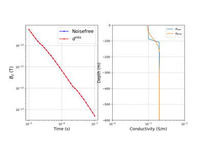
Time-domain CSEM for a resistive cube in a deep marine setting

Time-domain CSEM for a resistive cube in a deep marine setting

EM: TDEM: 1D: Inversion

EM: TDEM: 1D: Inversion

Heagy et al., 2017 1D RESOLVE and SkyTEM Bookpurnong Inversions

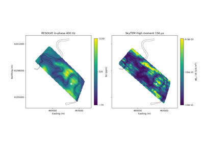
Heagy et al., 2017 1D RESOLVE and SkyTEM Bookpurnong Inversions