SimPEG.electromagnetics.frequency_domain.sources.MagDipole#
- class SimPEG.electromagnetics.frequency_domain.sources.MagDipole(receiver_list, frequency, location=None, moment=1.0, orientation='z', mu=1.25663706212e-06, **kwargs)[source]#
Bases:
SimPEG.electromagnetics.frequency_domain.sources.BaseFDEMSrcPoint magnetic dipole source calculated by taking the curl of a magnetic vector potential. By taking the discrete curl, we ensure that the magnetic flux density is divergence free (no magnetic monopoles!).
This approach uses a primary-secondary in frequency. Here we show the derivation for E-B formulation noting that similar steps are followed for the H-J formulation.
\[\begin{split}\mathbf{C} \mathbf{e} + i \omega \mathbf{b} = \mathbf{s_m} \\ {\mathbf{C}^T \mathbf{M_{\mu^{-1}}^f} \mathbf{b} - \mathbf{M_{\sigma}^e} \mathbf{e} = \mathbf{s_e}}\end{split}\]We split up the fields and \(\mu^{-1}\) into primary (\(\mathbf{P}\)) and secondary (\(\mathbf{S}\)) components
\(\mathbf{e} = \mathbf{e^P} + \mathbf{e^S}\)
\(\mathbf{b} = \mathbf{b^P} + \mathbf{b^S}\)
\(\boldsymbol{\mu}^{\mathbf{-1}} = \boldsymbol{\mu}^{\mathbf{-1}^\mathbf{P}} + \boldsymbol{\mu}^{\mathbf{-1}^\mathbf{S}}\)
and define a zero-frequency primary simulation, noting that the source is generated by a divergence free electric current
\[\begin{split}\mathbf{C} \mathbf{e^P} = \mathbf{s_m^P} = 0 \\ {\mathbf{C}^T \mathbf{{M_{\mu^{-1}}^f}^P} \mathbf{b^P} - \mathbf{M_{\sigma}^e} \mathbf{e^P} = \mathbf{M^e} \mathbf{s_e^P}}\end{split}\]Since \(\mathbf{e^P}\) is curl-free, divergence-free, we assume that there is no constant field background, the \(\mathbf{e^P} = 0\), so our primary problem is
\[\begin{split}\mathbf{e^P} = 0 \\ {\mathbf{C}^T \mathbf{{M_{\mu^{-1}}^f}^P} \mathbf{b^P} = \mathbf{s_e^P}}\end{split}\]Our secondary problem is then
\[\begin{split}\mathbf{C} \mathbf{e^S} + i \omega \mathbf{b^S} = - i \omega \mathbf{b^P} \\ {\mathbf{C}^T \mathbf{M_{\mu^{-1}}^f} \mathbf{b^S} - \mathbf{M_{\sigma}^e} \mathbf{e^S} = -\mathbf{C}^T \mathbf{{M_{\mu^{-1}}^f}^S} \mathbf{b^P}}\end{split}\]- Parameters
- receiver_list
listofSimPEG.electromagnetics.frequency_domain.receivers.BaseRx A list of FDEM receivers
- frequency
float Source frequency
- location(
dim)numpy.ndarray, default:numpy.r_[0., 0., 0.] Source location.
- moment
float Magnetic dipole moment amplitude
- orientation{‘z’, x’, ‘y’}
or(dim)numpy.ndarray Orientation of the dipole.
- mu
float Background magnetic permeability
- receiver_list
Attributes
Location of the dipole
Amplitude of the dipole moment of the magnetic dipole (\(A/m^2\))
Magnetic permeability in H/m
Orientation of the dipole as a normalized vector
Methods
bPrimary(simulation)Compute primary magnetic flux density.
hPrimary(simulation)Compute primary magnetic field.
s_e(simulation)Electric source term (s_e)
s_eDeriv(simulation, v[, adjoint])Derivative of electric source term with respect to the inversion model
s_m(simulation)Magnetic source term (s_m)
Galleries and Tutorials using SimPEG.electromagnetics.frequency_domain.sources.MagDipole#
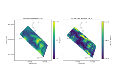
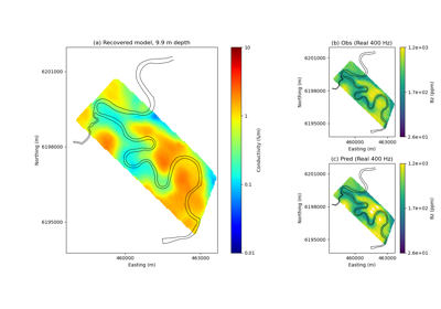
Heagy et al., 2017 1D RESOLVE and SkyTEM Bookpurnong Inversions
Heagy et al., 2017 1D RESOLVE Bookpurnong Inversion
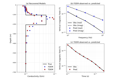
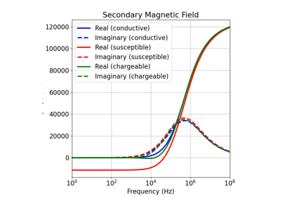
1D Forward Simulation for a Susceptible and Chargeable Earth